Hello Quentin:
I have made a quick model for you to look at, simulating version “a” of the figure you’ve attached.
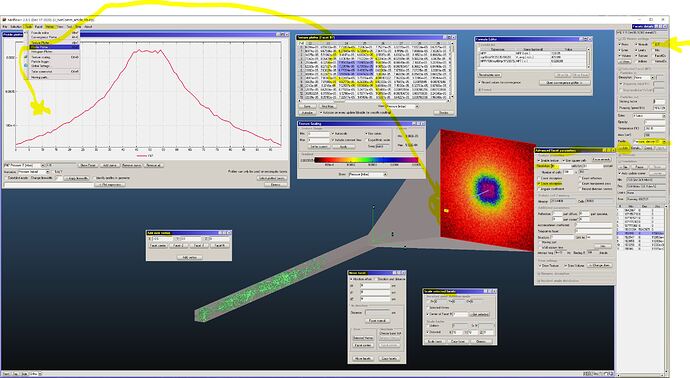
It is a 1cm2 tube, 30 cm long (the same ratio as in the paper), and placed a 10x10 cm2 screen at 20 cm from the end of the tube, see the attached figure
The tube has been made by starting from scratch and creating 4 vertices (“Vertex” menu) then I have used the “Create facet from selected” in the “Vertex” menu (Alt-V shortcut on the keyboard) to create the facet. I have then used the “Extrude” command in the “Facet” menu, by extruding 30 cm length.
Facet no.1 is centered at the origin of the XYZ frame of reference.
I have then copied the first facet, no.1, and moved it 20 cm in the +Z direction using the command “Move” in the “Facet” menu.
Next I’ve made it 10x bigger, using the “Scale” command, again “Facet” menu, and selecting the option “Center of face # 7” (you must enter the number of the facet you want to scale).
Next, I have created the 4 side facets of the truncated pyramid made up by facets 7-11 (plus facet 1)… and set the sticking coefficient of 7-11 to 1 (so that they do not bounce back into the system, which is not what you want to simulate).
I also changed the opacity of facet no.1 to o, so that the molecules do not bounce on it (it is the “exit” of the system. I have set facet no.6 as the desorbing one, setting cosoine as desorption type and 1 (mbar*l/s) the total outgassing (you can change that to any number you want).
I did not simulate the cube on the left of the figure in the NatComm paper since I know that the effusion from it into the tube is a cosine distribution, but I could have done it easily… only drawback is that the simulation would be slower because it would spend a fraction of the time making molecules rebound inside the cube instead of diffusing along the tube.
I have then set some colored textures on the “screen” (facet no.7) in order to visualize the distribution of the impinging molecules (which gets stuck on it since I set sticking=1).
I have set the texture size to “10” units in the “Advanced facet parameters” window ("<<Adv" button on the right, see other smaller figure.
As you can see I have also set a “pressure profile” on the same facet, by choosing the option “Pressure,. density (u,v)” on the pull-down menu on the right of “<<Adv” button… so that it shous on the “Profile plotter” (see figure) the projection along the “u” axis of the textured facet no.7.
The “u” axis is the horizontal edge of the facet, by the way, if you select the “v” option you’d get the projection along the vertical edge of the square facet no.7.
You can visualize the (u,v) local axis of any facet by selecting the facet (clicking on it with the mouse or on the list of facets on the right) and then checking the box “u,v” at the top right of the screen.
The “Profile plotter” window is opened by selecting it in the “Tools” menu.
Same for the “Texture plotter” which you see as a table of numbers. It is the pressure values in each of the texture elements, you can copy it with the mouse (right button to “copy” after selecting with left button). I have highlighted a 2x4 section of the texture matrix for you to see.
If you right0-click with the mouse on the tiny “v/u” cell in the uppermost left corner of the texture plotter table you can copy all or only the selected data, which you can then paste into Excel or other program to plot the textures.
Do not forget to save the file in the “File” menu!.. and do a “Ctrl-S” (shortcut for “Save”) from time to time, as the program may crash and there is no “undo” button for most of the commands (some do have it, though, and sometimes soon all of them will do).
Hope it helps, if not write back.
Good luck!

