Appropriate Use of Time-Dependent Simulations

[JEickman (Joey Eickman)]

Hello,

I’ve just started using Molflow and am trying to understand what scenarios can be evaluated with time-dependent simulations. There is some conflicting information based on other forum posts I’ve read.

Some responses say Molflow should only be used to simulate phenomena that last a few seconds, whereas others say it can simulate hours-long problems. Is the issue with simulating longer problems concerning the accuracy of the solution and the required computational expense?

I’ll describe the problem I am looking to simulate and maybe someone can recommend the correct course of action.

I want to evaluate the evacuation time of a chamber which is approximately a 7m long cylinder with a diameter of about 2m. This simulation would consist of two phases. First, gas is puffed into the chamber by a time dependent offgassing profile up to about 3e-3 Torr. Then the pumps turn on and evacuate the system down to 1E-9 Torr. I want to evaluate how long it takes to reach the desired pressures for different pump speeds and offgassing rates. In general, the evacuation needs to happen within 5-10 minutes.

Is this type of problem and time scale appropriate for a time-dependent simulation, or should I use Molflow to inform my solution based on analytical calculations as described in this forum post?

Question: Calculate pump time

Dear Tobi, One of the core principles of Molflow is that in can only generate, reflect or absorb molecules on surfaces (and not in the volume). This is the reason that you can't set a starting pressure: that would require recognizing "valid" space between the facets and uniformly fill it with initial particles. In theory, you could create such an initial condition by injecting some particles for a very short burst (controlled by parameters, as described in the time-dependent mode), closing inj…

Thank you,
Joey

[maarton (Marton Ady)]

Hello Joey,

Molflow calculates all molecule bounces until a desired time. Because of this, it’s not the actual physical time that is limited, but the number of hits to calculate. For example, your 7m long, 1m radius geometry would need the same computing time to simulate 100s of physical time as a 7cm long, 1cm radius system would need for 1s (the number of hits would be the same).

I believe the 5-10 minutes is certainly feasible - you can increase statistics by choosing larger time windows (so more hits are captured for each moment).

My feeling is that a 7m/1m geometry has almost immediate dynamic response, since it has good conductance, so your pressure will be governed by the changing input and the changing pumping, not by molecules needing time to readjust.

Good luck and let me know if need help to set up the simulation,

Marton

[rkerseva (Roberto Kersevan)]

Hello Joey:
You can certainly simulate up to several hours, especially if your geometry is as simple as you’ve described it here.
You need to use variable-length time moments, so as not to lose the details of the exponentially-decaying pump down.
I’m travelling right now with very poor internet connection, couldn’t connect my laptop using the cell phone as hotspot, so if you can wait 2-3 days that I go back home I’ll be happy to show it to you here, posting the file.
Cheers, and good luck in case you go on your own.
R.

[alan (Dr Alan Van Drie)]

I had a question to better understand what you are trying to do. It sounds like you are puffing in gas and then have a seperate outgassing source. Is this correct? I assume outgassing will be water while the puff gas is something else?

To do a gas fill I would do a very short puff. Short means much shorter than your characteristic pump down time given by tau=Vol/Speed. This should fill the chamber evenly unless your pump speed is very very large.

There are somethings to consider 1) At 3E-3 Torr you are in the transitional flow regime not molecular which is what Molflow simulates. However, I’m guessing it probably good enough as I assume the chamber will spend most of the time in molecular flow. 2) Does your pump have a pressure dependent speed? What type of pump will you be using.

Personally, it sounds like your system will always be in quasi-equilibrium (7m/speed of particle << tau), so the pressure through the vessel is the same. In which case it would be easier just to use a program like Vactran to get pump down curves. Pump down is just a simple first order differential equation with a constant outgassing and maybe a pressure dependent pump speed so any software like Excel, python, and etc… could be used too. Most outgassing is time dependent, but over 5 mins I would probably just use a constant value.

Best,
Alan

[JEickman (Joey Eickman)]

Thanks everyone for the timely responses.

I’ve constructed a few models and found that pumping out the initial gas puff does not take long at all; assuming we have 2 cryopumps with 5000 L/s pumping speed for hydrogen it takes around 30 seconds depending on pump location. The real battle is reaching very low pressures (1e-9 Torr) while the whole vessel is outgassing.

To evaluate this, I’ve made a few different configurations of the geometry and used Molflow to apply outgassing to all the internal surfaces and pumping at specific locations. Molflow will report the final outgassing rate and pressure in the vessel. This allows me to calculate the effective pump speed with P = Q/S_eff.

I can use that S_eff to estimate the pumpdown time for an initial gas puff using:

t = -V/S_eff*ln(P/P_0)

However like I mentioned, the transient pumpdown is not very interesting for this case. The utility of using Molflow for this is to get an estimate of S_eff for different geometries and the minimum steady state pressures that can be reached given specific outgassing rates from the vessel. Here is a screenshot of one of the models I’ve been working with

Please let me know if there is any flaws in my methodology or if there is more analysis I could do to get a better result. I’m also wondering about the best way to simulate multiple species of gas. So far, I’ve only assumed hydrogen outgassing, but in reality there will be water and other impurities. Is it best to do multiple simulations for each species or to try and combine them and averaging their molecular mass?

[rkerseva (Roberto Kersevan)]

Hello: your methodology is OK, but rather than using an estimated time for pumpdown from the analytical equation you can actually SIMULATE the whole pumpdown, over the time length that you need.
Since I do not have your detailed geometry, I’ll attach a sample file with time dependent calculations. In a real case you could even simulate the time dependent outgassing, if you can estimate it, by using the built in feature of a parameter file, and assigning it to all facets with time’dependent outgassing. Like this you can simulate the initial exponential decay (as per your equation) and then the 1/t pumpdown due to thermal outgassing (decreasing as 1/t) plus another phase proportional to 1/sqrt(t) (like water desorption)… and finally you may even add a constant outgassing at some locations (like permeation or leaks, virtual or not).
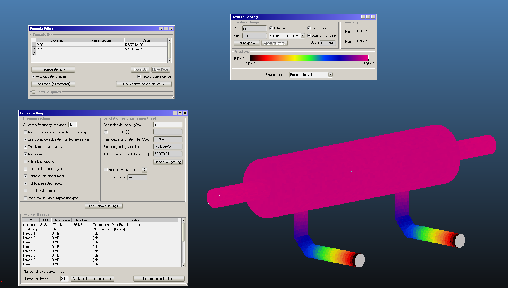
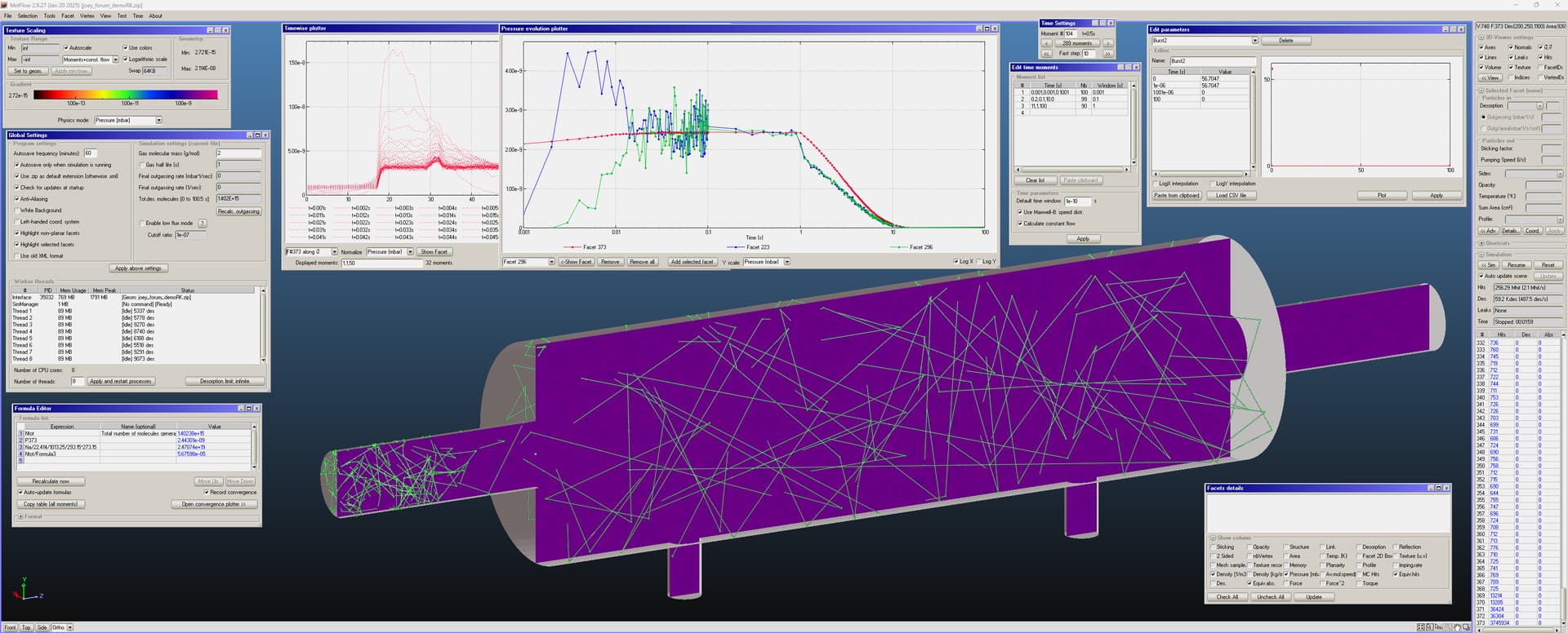
Here you can see a screenshot of the model I have made just looking at your screenshot, a 7x2 m cyl with 2x 5000 l/s pumps (connected via different geometry as compared to yours, for simplicity).
I send also here the link to the time-dependent simulation, the file makes 21 MB, so I can’t put it in attachment here, it’s a Dropbox link:

https://www.dropbox.com/scl/fi/tzrjdpyskelfdfo129zk9/joey_forum_demoRK.zip?rlkey=caprrs4vwn93b8lq14apthn8k&dl=0

Hope it works.
As you can see on the screenshot, I have defined a number of different length time periods (moments): I start with very short ones, 0.001s, up to 0.1 s (100 of them), thjen I go to 0.1 s interval, from 0.2 to 10 s (99 total), and then finally 1s interval from 11 s to 100 s (90 moments).
On the “pressure evolution plotter” you can see the average pressure evolution over 3 facets, namely: facet #373, which is the coloured one on the figure (a 2’sided, transparent facet, textured with texture size 5x5 cm, squares).
Then there are facet #223 and 296, which are the two PUMPING facets.
The outgassing I have set ONE facet only, a “burst” of 1E-6 s times 56.7047 mbar*l (See “Edit parameters” window on the upper right. I have taken this value from your screenshot, just to get ballpark numbers correct (although my geometry is not exactly yours). The desorbing facet is #147 (i.e. the end-cap of the bigger cylindrical body with a hole in the middle, on the left on the figure).
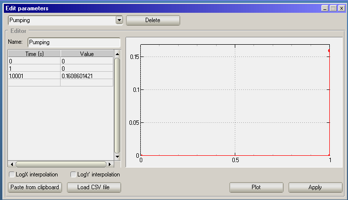
I have also defined a parameter call “Pumping” which sets the sticking coefficient of the two pumping surfaces to 0 until t=1 s, then it suddenly switches to the value corresponding to 5000 l/s for H2 gas, see the other figure here.

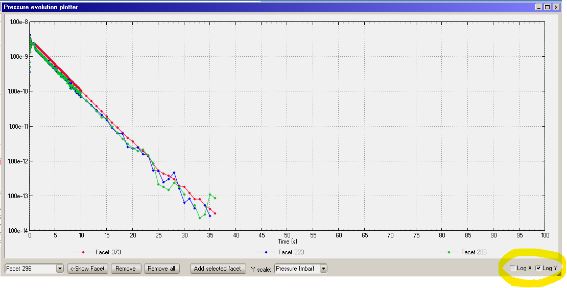
As you can see on the “Pressure evolution plotter” window the pressure starts from 0 (logical), then it increases, with an overshoot on facet #223 (blue line) nut then all 3 lines go to the same value, around 2.45E-9 mbar immediately before the pumping starts (1 s).
The 3 pressures then decrease in with separate curves, but if you look at them on a lin-log scale they have PARALLEL paths, and the linear (on a log vertical scale) slope is proportional to the S*t/V exponent in your formula… apart from the initial time when there is no pumping, of course.
See the third figure for “Pressure evolution plotter” in lin-log scales, here:

The advantage of this way of simulating the thing is that in principle one could have a time-dependent outgassing, as I said, and therefore one would have non constant slope on this graph.

I see now that the order of the figures is not correct, sorry… it is 2,3,1 as referenced in the text.

I stop here, if you have further questions or remarks to make please write back.

Cheers, and good luck.

R.