I have a section of pipe with a fairly uniform density, but I know my results are not really correct since it is in transitional flow regime and it really effect my results. I was trying to think of a way to hack collisions within molfow.
I think you could do it using a set of orthogonal facets that are completely sticking and with outgassing proportional to the flux in and that are spaced at the collision length, but that sounds like a lot of work to iterate on many facet to get it to converge to a pressure consistent with the collision length.
If I had a transparent plane that could scatter particles but not stick also spaced out to the collision length would be a bit easier. If you did a 50%/50% transparent plane and space them out 2x the collision length would give too much weight to the back scattered and not forward scattered particles.
I think a more simple hack would be to define a collision length for a defined structure that you can reasonable expect uniform pressure in based on an initial pressure profile without collisions. When ever a particle enters that structure you can randomly scatter the particles trajectory. After you run with collisions you can see if the pressure changes and change the collision length to match the new pressure. Iterate through this process until it converges to having a consistent pressure and collision length. I assume with the CLI you could write a script to automate this. If you start to get a pressure gradient within the structure you will have to sub divide it further and start over for each section.
Thanks Alan for the suggestion, but after discussion with Roberto frankly, we won’t add it.
Three reasons:
The iteration is somewhat feasible in case of parameter changes (which are scriptable), but becomes almost impossibly laborous in case of geometry changes (you would need to update surface positions to match the collision length)
The random scattering on the virtual surfaces would need to be position-dependent: typically in case of gas injection from an orifice, the gas diverges from the axis in case of non-molecular flow. That would mean that we need to define an axis, and we try to avoid breaking the geometry generailty in Molflow (one exception was the “moving parts” feature, where one can define a rotation axis).
Practical: currently only I am adding new features in my “free time”, so I’m focusing on keeping the code alive (bug fixes and devops). The most requested feature is iterative simulations (for surface saturation, mainly NEG coating and cryogenic). Here in the accelerator world we barely have viscous flow calculations.
Also, Roberto is unsure how much you could trust the results after these approximations. And benchmarking with experimental data would be a large project, probably not supported on our side without a practical application in sight.
Sorry for the negative answer, and hope that if iterative simulations will be implemented, you’ll find a use for it as well (outside of viscous flow).
I’ve been able to hack a scatter plane using a combination of planes with certain reflection and teleportation properties. The scattering will be whatever you can set in molflow: Uniform, Cosine, or Cosine^N. Initially I was thinking you set the gap between these scatter planes to be equal the 1D mean free path and then adjust the gaps to be consistent with the density. However, you can keep the gaps between the planes fixed and smaller than the shortest mean free path, and instead adjust the scatter plane’s transparency (opaqueness) to make make the mean free path effectively longer than the gap spacing. I assume one could parameterize the opaqueness so a script could adjust this value to converge on consistent effective mean free paths and density values?
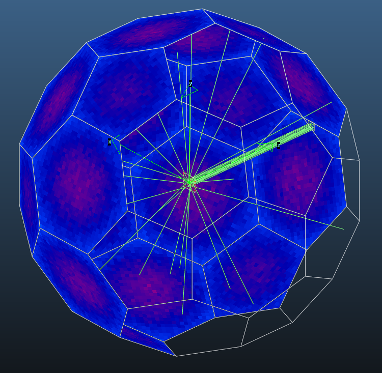
There are papers on particle in cell DMCS codes that model transition flow to compare too. They compare their code to both analytic models and experimental results so it’s a great resource to use with minimal work to compare a simulation done in Molflow. I’ve attached an image of a beam scattering uniformly off one of these planes. When I have more time I will try a simple geometry from one of these papers and compare.
Usually particle in cell codes will have a collisional operator, and it made me wonder what the angular distribution of the scatter particles should be to replicate physical results. For less than 1 eV, particles will mostly elastically scatter off the Lennard-Jones potential, which will have some distribution different than what you can set for facets in molflow. However, so long as the particles are Maxwellian (isotropic) it will average over many collision in a long enough time window to also be isotropic. So that’s why I think a isotropic (uniform) scatter plane will be able to give appropriate averaged results. Actually, any scattering type should average out over time to be isotropic to match the input maxwellian distribution, so I don’t think it probably matters.
I also don’t really understand why you need to define an axis. You just need to have the scatter plane geometry to match your density iso-contour lines. In the case of a pipe it easy since the density gradient doesn’t change direction. However, for an aperture it may change with density so this hack may not be simply implemented. Now you could have a 3D set of smaller orthogonal planes to replicate an “equivalent” particle in cell geometry in this case, but it would be a lot of work to setup the geometry. However, once you have it setup you can cut and paste into any model. Eventually, I’ll learn how to use a subset of OpenFOAM to properly model transition flow, but my hack may work for simpler geometries in Molflow.
Another way scattering may be done with only one facet would be to set the desorption on both sides of facets equal to its adsorption (with SF=1). Can you change these in a script? The downside to this approach is that you would have two iteration loops. The first is to converge on consistent adsorption and desorption on all surfaces, then again to iterate over transparency to converge on a consistent mean free path/density.
Who knows, just like my density hack got you guys to implement my facet density formula, maybe you will implement a better structure/trajectory scattering/script solution This work I’ve done so far is my “free time” too so I understand, lol.
Just a small feedback that despite the lack of reply, we are considering what you wrote and we plan to add a basic support for collisions early next year. Our chemistry lab does plasma sputtering, and they used Molflow to have an idea of where the sputtered particles coming from the cathode will end up.
Of course, Molflow doesn’t take into account the collision with the low-pressure gas, and this is something they requested us to add. The good news is that it’s an internal request so now there is justification to spend time with the implementation. We’ll brainstorm a bit on how to do it (user-defined scattering distriubtions? Hard-sphere collision model with a given gas pressure?) and will ask for your opinion before adding the feature.
This is tough. The only way to do it is to have the equivalent of PIC code. In this case a matrix of the cells facets instead of the cell volume itself. Then you would have to iterate the simulation adjusting the density each time until it converges to a steady state value. I think you could get away with fewer facets if you make it adaptive to be perpendicular to the density gradient with an equivalent 1D diffusion scale length in the direction of the density gradient??? Think 2D shells for the 3D geometry, or 1D for 2D geometry.