I use piezoelectric valve to inject hydrogen gas to Tokamak device.
here gate valve of pumps is open. and when this prefilled gas is thought to be diffused enough to make equilibrium state, plasma discharge is started.
So, it’s very transient situation which all process is done within 200ms from gas injection to end of plasma discharge.
I have already made modeling and it fits quite well to the real experimental case.
But, in pipe between piezo valve and main chamber, it is clear (by calculation of its Knudsen number) that it’s going through laminar(viscous) flow region. An I think little gap between experimental and simulation comes from here.
here, I want to know how much error is made from this flow transition.
or I want to know if there is any guideline of recommended pressure range.
First of all, well done for successfully setting up a time-dependent simulation, which is quite hard.
Unfortunately the problem you mention is - to our knowledge - unsolved. When expanding from high pressure to molecular flow, we go through three regimes, and each of them have different physics (fluid dynamics, laminar flow then free molecular flow). Molflow doesn’t check the regime, it assumes free molecular flow, and scales pressure linearly (meaning you could enter 1 million bar*l/s and results would simply be scaled up).
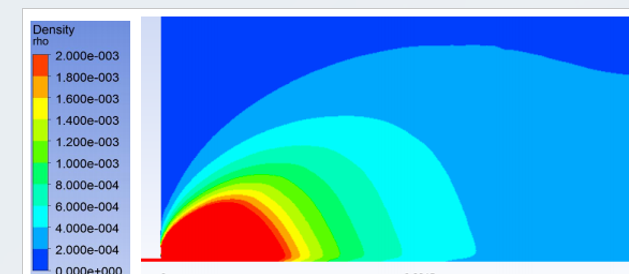
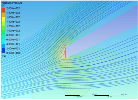
For a gas jet device, what I did was to use a colleague’s fluid dynamics simulations from a CFD code (ANSYS) to get the streamline and the pressure contour:
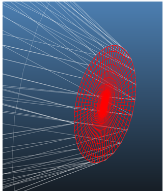
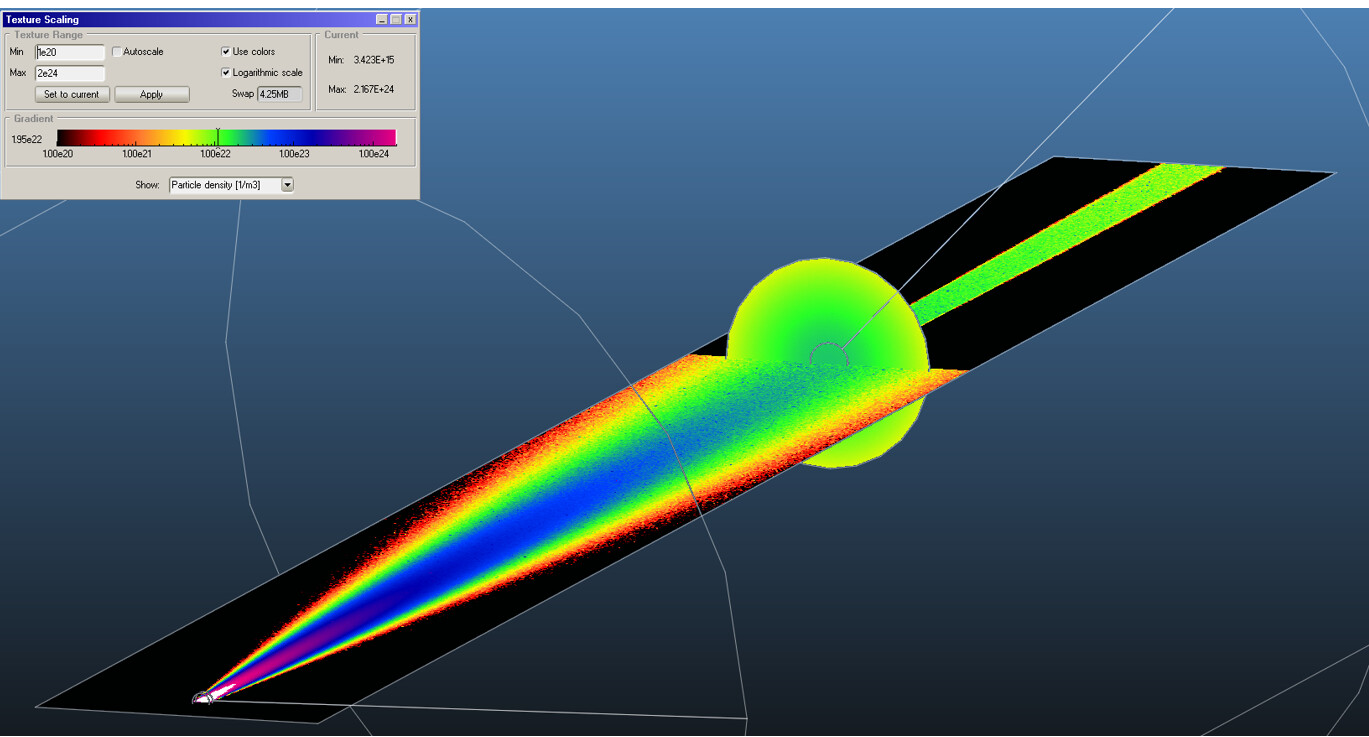
Then create a desorbing surface at the viscous-free molecular boundary, and set it as desorption surface in Molflow:
When this is time-dependent, it’s probably not possible, as the boundary itself would move in time.
Therefore, in your case, I would probably keep doing what you do, but I can’t give an estimate to the error. This problem is most likely solved somehow in the space industry where high-pressure discharge to vacuum (rocket propellent to space) needs to be simulated.
Now that you have mentioned its property in linearly scaling ups,
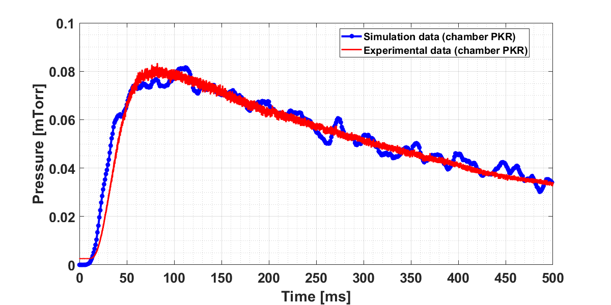
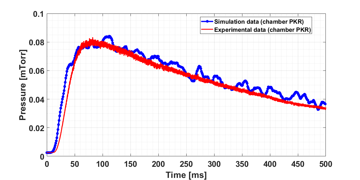
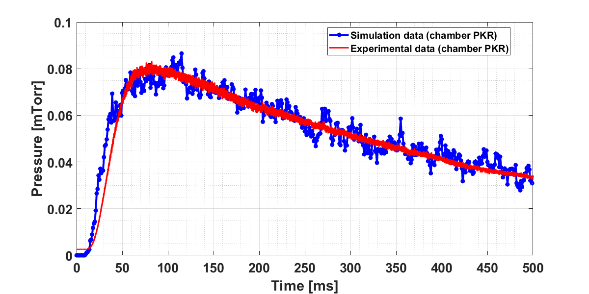
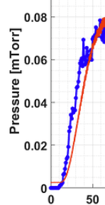
assuming it’s all in molecular flow region, would it be okay to simply adding its base pressure on simulation data to match real data like I did in pictures?
What do you think about smoothing simulation data in data processing?
The simulation I’m doing is quite large scaled and the target facet I’m trying to watch is pretty small I think. So, It takes too many time to converge and it shows too much flucuation as shown below. To complement this, I use smoothed data. whick one do you think is closer to realistic situation?
Yes, absolutely. Your pressure burst is over the background, and you can simply add the two. We regularly do simulations for different gas types one by one, then sum the results (which is the same logic as adding dynamic pressure to constant background).
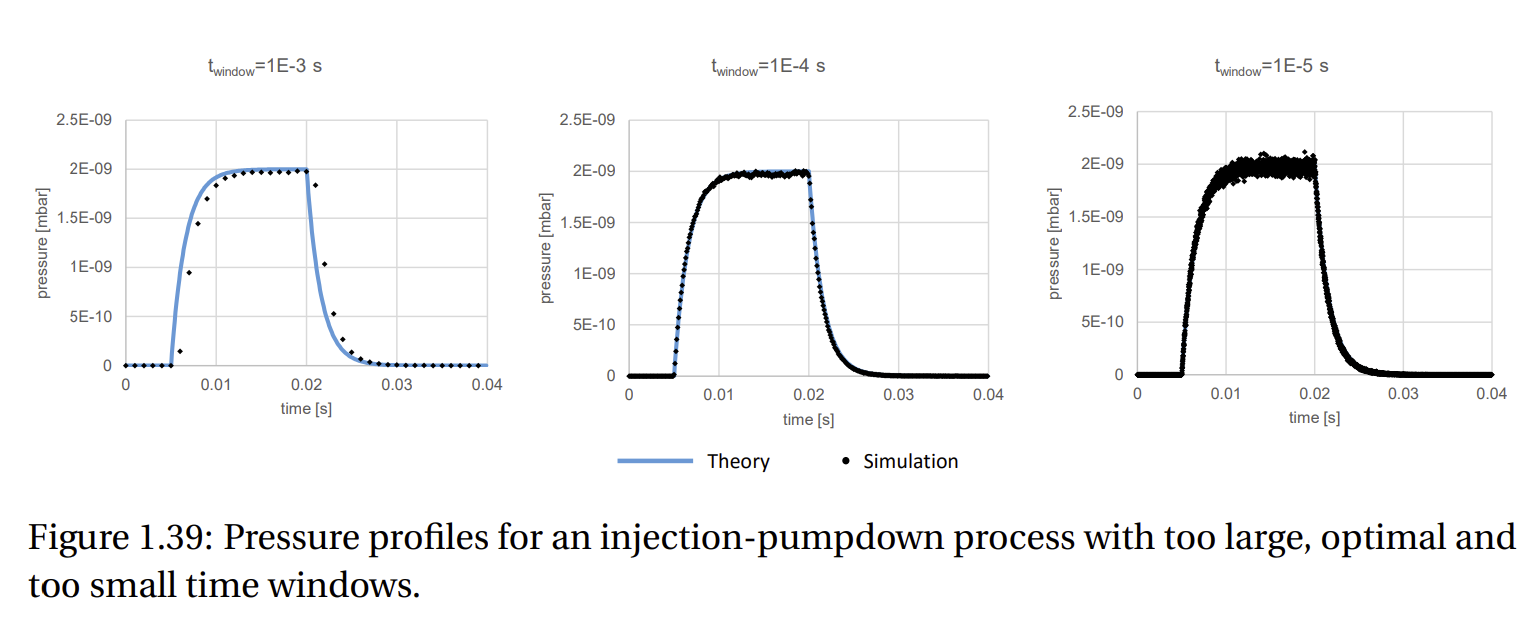
By choosing a larger time window, you lose “dynamic resolution” but gain statistics. In my Phd thesis I showed an example:
You can see that increasing the time resolution reveals fast changes, but adds noise.
In your case there is no physical reason for the fluctuations on the blue curve, so clearly the smoothed data is the true one, but smoothing introduces a delay, as we can see on your curve:
The rise is lagging behind.
Luckily, Molflow allows to set different time window sizes for different moments: n your case, keep the current time window until ~100ms, and then increase it signinifcantly for the slow decay from 100ms.