How is the time dependent outgassing profile sampled?

[alan (Alan Van Drie)]

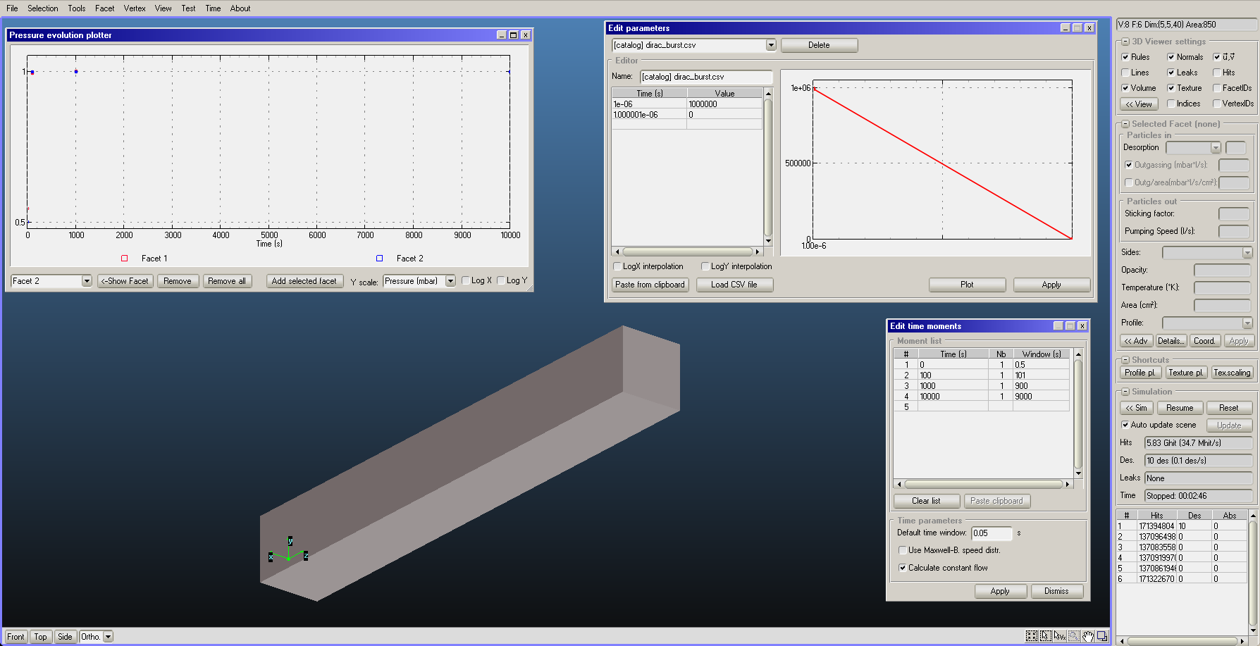
I recently was using molflow to estimate the volume of some complex geometries in my model…used for estimating rough out times in VacTran software. I do this by creating a profiles whose area under the curves gives a fixed amount of 1 mBarL of gas. Divide this by the calculated pressure and you get the volume. However some things I noticed made me question how the time dependent outgassing profile is “sampled”.

Initially I didn’t have any pumping surface, so only 10 particles are generated, one for each thread, and do those 10 give you a good enough “representation” of the outgassing rate profile used to give the correct rate integrated 1 mBarL of gas. If you add just a little amount of pumping then you can generate more desorbed particles to better represent the profile, but not so much that it effects the pressure on short enough timescale. However, it would still be useful to know how you do this so a better choice in profiles is used.

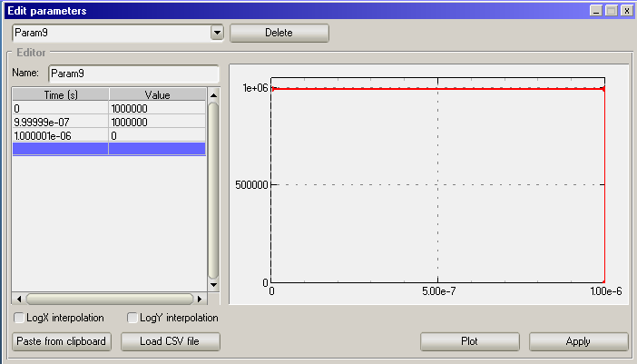
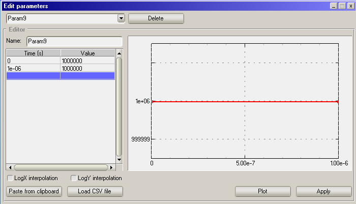
I also tried different profiles, to see how you might do this to see if I got bigger errors depending on the profile, but I really couldn’t tell because of a bug in the plotter; will not update MC counts after the 10 particles are generated. The one thing I did figure out is that the profile can be shorter in time than what you define in the moments…I though it had to include the longest time as defined in your moments even if it was just zero.

Lastly, your catalog dirac_delta profile injects 0.5 mBarL, I assume you where trying for 1.

Best,
Alan

[maarton (Marton Ady)]

The time dependent outgassing profile is integrated, since computers must have a cumulative distribution function to generate random numbers according to the PDF.

The problem is to construct an integrated desorption, which is in fact quite difficult if you allow the user to enter lin-lin, log-lin, lin-log and log-log parameters:

Here is the source code, and I explain what it does: src/Simulation/IDGeneration.cpp · master · molflow_synrad / molflow · GitLab

Below, latest moment means the last user-defined moment in the Edit Moments window plus half the time window. (reason: if the last moment is 100s, and window is 1s, then we don’t care what happens after t=100.5s)

1. I sanitize the user input. If the user defined the first moment after t=0, then I constant-extrapolate the first outgassing value to t=0. Also, if the “latest moment” is between two user moments, I interpolate a value there.
2. I divide each section to 10 subsections. A section is the time between two user-defined moments. In case of linear time, these are equal, in log, they are log increasing.
3. I do a poor man’s integration of each section by adding the molecules desorbed in each subsection (1/10th of the section). This could be done better by analytically integrating the interpolated function (a linear line in PDF becomes a second-order spline in the CDF) - there are analytic integrals for the lin/lin, log-lin and log-log cases, but no closed form for lin-log.
4. I generate a random number and look it up in the CDF, therefore choosing desorption moment. The generated molecules will follow the user-defined distribution.

I’m almost sure that the problem with your file is that you define a time-dep outgassing but don’t define moments, and do a static mode simulation (!). This would still work but would display the pressure in t=infinity assuming there is sticking somewhere in the system. Molflow simply chooses the outgassing at t=infinity in static mode, which is 0 in your case, but molecules can’t get out of the system and contribute to a false pressure. This “no time moments and no sticking” is an edge case that Molflow wasn’t designed for - molecules get stuck.

About the Dirac burst

You can check in the global settings this field:

It shows that the latest moment is 5E-11s (half of default time window 1E-10), meaning molecules are not desorbed after that. I’m sure this is causing the Dirac burst injecting half the desired gas, because the way it is defined in Molflow is correct:

• Injection at Q=1E6 from 0 to 1E-6, injecting 1mbar.l
• Rapid cutoff from t=1E-6 to t=1.000001E-6s

By the way, in your other post you write that catalog parameters can’t be used for outgassing - you could use it in the end, couldn’t you? Or how did you get the 0.5mbar.l?

I suggest you to upload here or send me your file (replace the confidential geometry with a cube for example) and I’ll debug. Well, after the Easter break.

[alan (Alan Van Drie)]

This is strange…your dirac_burst.csv should give 0.5mBarL of gas since you have a triangle shape profile A = 1/2 BxH Q=1/2 1E-6 sec x 1E6 mBarL/sec = 0.5mBarL, but my simulation results implies 1mBarL. Something is wrong. Using 2.9.8 beta on a MacBook Pro M1.
Volume Test 3.zip (56.9 KB)

What is wrong is me, lol. The confusion for me comes from how you plot vs how you interpret back to t=0 that is not shown in the plot. The plot it looks like a triangle, and my brain saw the 1E-6 and 1E6 and made the wrong conclusion. But it’s just a triangle from 1.000000e-6 to 1.000001e-06 which are just the two points you explicitly define which gets plotted. If you include the implicit point at t=o explicitly then it look like a nice step function and is less confusing.

Technically below is exactly 1.0000000 mBarL

I think you should explicitly make people define a t=0 point so they don’t accidentally get a profile different from what they think they defined because they didn’t realize how you interpret back to t=0. Is this documented anywhere?

This also begs the question, how do you interept beyond the last point in the profile. Do you assume it’s zero or do you assume it’s the same as the last point. Ran below profile and it seems to be the later case; assume it’s the same as the last point.