Dear Andreas,
Monte Carlo simulations are advantageous because they solve physical problems by billions of random events. However, when the results aren’t as expected, they are inherently difficult to debug because one cannot follow all random events - plus they are not perfectly deterministic either.
Concretely, the system of Thomas, while simple in physical sense, is still somewhat complex, for example there is a net gas flow towards the exit, making the ideal gas equation not (fully) valid - pressure is not isotropic, it will be higher in the flow direction.
So instead of comparing MolFlow with the papers that you refer to (thank you very much), first what I recommend instead is to debug the “building blocks” of the simulation. If we agree, then we can discuss why the results are not as expected. Credit must be given to Thomas for his Excel sheet, that takes a Maxwellian distribution as initial state and applies the thermal accomodation coefficient thorugh a hit with the wall, that we hope agree that has the form:

where Ei is the energy of the incident molecules, Er is the energy of reflected molecules, Ew is the energy which would be carried away by all reflected molecules if the gas has had time to come to thermal equilibrium with the wall (I.e. “wall energy”).
I slightly modify the sheet as follows:
- I don’t calculate A_TAC=0% and A_TAC=100%, since it is clear that the results are Maxwellian: in the 0% case the initial Maxwellian distribution is not modified, in the 100% case the distribution is always perfectly rethermalized by the wall (default setting in MolFlow, confirmed to be Maxwellian)
- For the “in-between”, instead of a range of A_TAC from 10% to 90%, I only calculate for 50% as a representative mid-value.
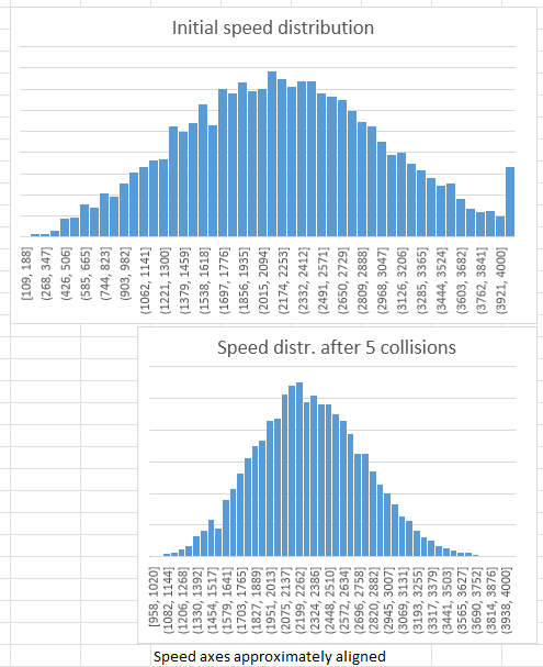
- He has calculated the v_rms, I also calculate v_mean and the speed distribution
- He has calculated the new distribution after one wall collision, I continue for several collisions.
- I increase the number of simulated particles to 10000
The results speak for themselves (Excel attached molflow_5_collisions.xlsx (5.3 MB) ):
You can see that simply by executing 5 wall collisions, in a way that Thomas himself set up, the speed distribution changes. This is not MolFlow running, this is simple repeated execution of the acc. coefficient to get a new random speed - using Excel’s random() function.
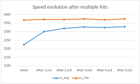
At this point, your kind feedback is welcome why - executing a well known mathematical formula - the speed distribution changes, and the average speed increases (while v_rms is constant except some statistical fluctuation - showing that the energy of the gas is constant).
If the calculation, based on Thomas’ Excel sheet is correct (as I believe it is), we have just proven that it is reasonable to switch from Non-Maxwellian to Maxwellian back and forth. If I have made a mistake, either in the Excel sheet, or somewhere else, your input is welcome to find it.
Regards, Marton
 .
.