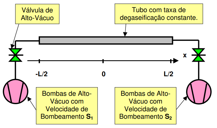
Its a cylindrical pipe with diameter in 3 cm and length 400 cm, which have a 2 different pumping speeds in the ends. These 2 speeds in 400 and 100 l/sec, so both need to increase temperature in the ends to reach these speeds, because their areas is about 7 cm2. There is my first question: I am right doing this or I missed something?
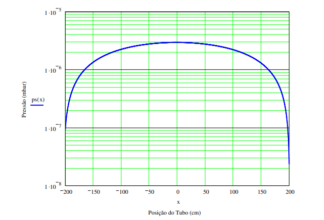
At first I simulated the system admitting sticking factor is 1 on both ends but the pressure profile does not fit with the theoretical curve using the diffusion equation for pressure.
Here is the first curve I obtained from Molflow, assuming sticking factor 1 on both sides. Using 430.15 K to reach 100 l/sec and 6800.15 K to reach 400 l/sec.
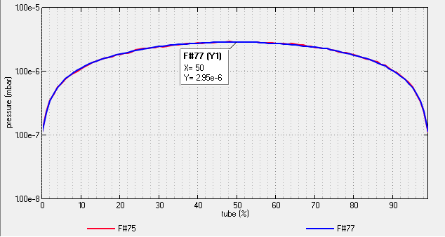
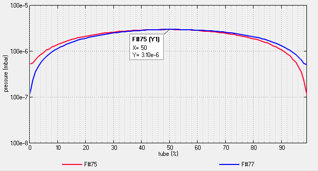
At second attempt I tried disregarding the sticking factor 1 on the 100 l/sec side and using the same temperature on both ends. This decreased the sticking factor to 0.25.
Here is the second curve I obtained along the pipe.
The second and my last question is what i’ve done wrong? I consulted my professor and we do not can imagine what happened wrong. Maybe I I misunderstood the sticking factor or basic vacuum formulation and concepts. I just need a little help
I am sorry if there is some confused words in my text, english is not my first language and I’ll be very thankful if you can understand my issue.
At all, I wish everyone good work and good research ^-^
“These 2 speeds in 400 and 100 l/sec, so both need to increase temperature in the ends to reach these speeds, because their areas is about 7 cm2. There is my first question: I am right doing this or I missed something?” - in molecular flow, the maximum pumping speed is not defined by the pumps, but the conductance, which for a 7cm2 area, N2 gas and room temperature, is around 77l/s. There is no physical way to go above that, even if you connect 100l/s or 400l/s pumps. Therefore I believe the exercise is incorrectly defined. (Setting the temperature on the pumping facets won’t have an effect on the pumping speed on the pipe.)
For the rest of your question, you played with the temperatures, which I assume is incorrect, as explained above. Please also note that at high sticking factors, pressure is not isotropical: it points towards the sticking facets, so profiles wouldn’t measure it correctly (pressure lower sideways than along the tube axis).
If you need further analyisis, please paste all parameters and the model and the equation. We can’t read a 366-page Portugese thesis to get the data.
A 3 cm ID pipe at 20 C, assuming the sticking is 1 at the end, has a maximum pumping speed of 311.3 l/s for H2, so your 400 l/s case is UNPHYSICAL. The 100 l/s case can be simulated assuming a sticking coeff. of 100/311.3=0.3212. If the gas is N2 then even the 100 l/s case is unphysical, the maximum value can be 83.2 l/s at 20 C for a mass 28 g/mole gas specie.
If the system you want to simulate is really like in the figure, with elbows and valves between the ends of the 400 cm-ling pipe and the pumps then you need to simulate that too, because the associated conductances will reduce the pumping speed of the two pumps. This means that the “equivalent” sticking coefficient at the pipe’s ends must be reduced compared to the one you obtained by dividing the pumping speed by the 3cm opening conductance (which is, as I said, 311.3 l/s for H2 and 1/sqrt(14) of this for N2, i.e.83.2 l/s).
I don’t understand why you change the temperature to get a different pumping speed (unless the system really has different temperature at the ends).
As Marton already mentioned, pressure is NOT a scalar quantity, it is a tensorial one, and its value depends on the orientation of the surface over which you compute it. This means that it is normal that the pressure calculated by Molflow+ is LOWER than that calculated via analytic equations near pumping surfaces, and the difference is bigger as the sticking coefficient of the pumping surface increases. In fact, it would be better to calculate the DENSITY and then convert it to pressure, since density is a scalar quantity. Molflow+ does the correct calculation for density, as explained in Marton PhD thesis (https://cds.cern.ch/record/2157666/files/CERN-THESIS-2016-047.pdf).
What outgassing coefficient did you use to get your pressure curves? Was it a uniform desorption along the 400 cm-long pipe? How did you model the two elbows and the valves? Unless we know the outgassing coefficient and its distribution along the pipe we can’t make the calculation on Molflow+ to help you out, sorry. Please provide the values, thanks.