Number of virtual particles

Hi, I am undertaking what promises to be a rather lengthy set of simulations--for CHESS-U at Cornell--where I will have to periodically read parameters from and write parameters to several hundred facets.  It seems that the easiest way to proceed is to read from and write to the XML file before and after simulations.  

I am able to use an XML parser to get values out using a Python script, however, when I try to compute the pressures on the facets using the folrmula provided in the user guide, I get a number that is off by a factor of 3-3.5 from what MolFlow reports.  I am guessing that this is because I used the number of desoprtions as the number of generated particles and this is not correct.  

I am guessing the number of particles generated is in the XML file somewhere but I do not see it.  Are you able to share some insight on finding this number or computing it from another parameter?  

Thanks!

Yev Lushtak

I have since discovered that I used R in mbar L rather than in J, introducing an error of sqrt(10).  However, the discrepancy varies slightly from facet to facet.  Having fixed the error, I still see a difference on the order of a few percent.  Therefore, if you are able to comment, that would still be very helpful. 

Hello Yevgeniy,

Sounds like a big undertaking, but if you already have a Python script to extract the info, let’s go ahead.

Since 2014 (Molflow versions 2.6 and later), there is no direct connection between the number of hits on a facet and the pressure. The pressure is calculated from the sum_v_ort value of the XML file (sum of orthogonal momentum changes per second).

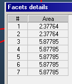
Wouldn’t it be possible to export the list of pressures (selecting all facets and using the Facet details window), since saving the simulation requires manual GUI interaction anyway?

If you decide to go ahead yourself, the formula to get the pressure is:

pressure = 1E4 * molecule_per_testparticle * (gasmass_gram_per_mole / 1000 / 6E23) *0.01 * sum_v_ort / facet_area

where

1E4 is the conversion of area (cm2->m2)
0.01 is the conversion of pressure (Pa->mbar)
Facet_area is area in cm, times 2 in case of double sided
Molecule_per_testparticle is totaloutgassingrate/nbDesorbed

​where

Totaloutgassingrate is the total outgassing rate of the whole system in Pa*m3/sec
nbDesorbed is the number of generated test particles (totalDes attribute of MolflowResults/Moments/Globsl/Hitss node)

As for a documentation of the current way physical quantities are calculated, check section 2.8 of the document “The algorithm behind Molflow”, in Documentation/Molflow documenation in the website.

Hi Marton,

Thanks for the detailed response, I will give this a go.  I will also take a look at section 2.8 of the algorigthms document. 

It is true that I could simply copy the pressures out of MolFlow.  However, I used this process as a way to familiarize myself with the MolFlow XML output and review using parsers.  Reading pressures this way will save a little time but not a tremendous amount, especially since I haven't coded an area calculation and I still ned to reference the areas calculated by MolFlow.

The real time saver will be being able to write the outgassing rates and the pumping speeds--as the system is conditioned by beam and the NEG pumping speed decreases--to the XML file since then I can just load the file and start the simulation.   

Great!

A few remarks about this:

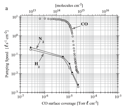
  • NEG conditioning cannot be simulated directly, as the pressure depends on the pumping speed and vice versa: the only way to approach this is your method, iterative simulations where after each step you update the sticking factor based on saturation. We did some brainstorming about this, and probably each simulation should represent a logarithmically increasing time step (conditioning is fast in the beginning and slows down). I believe what you really need is not the pressure but the number of pumped particles per area, and you can determine the pumping speed by interpolating in this figure:
    2019-02-18 09_57_20-Window.png
    (The source is this article
  • The good news is that you wouldn't need to apply the pressure formula above, you could calculate the impingement rate from the "nbHit" value in the output xml, multiplied by molecule_per_testparticle (see my previous comment), divided by facet area (see below). Then if you multiply this with the time step the simulation represents, you get the deposited molecules per cm2 during the time step, and that's what determines the NEG sticking
  • The difficulty in implementing iterative simulations this way is that you need to maintain a "saturation catalog", and after each time step (simulation) add the newly deposited gas quantity to the already absorbed quantity (in the previous steps)
  • I planned to add this iterative method automatically to Molflow, but ran out of time (it needs importing pumping speed curves, and some automatization, which is easy to implement numerically but is quite hard to integrate in the user interface). Such a feature might come in the future, if there will be a person to maintain Molflow (I'm quitting the project in a few weeks unfortunately)
  • I could, however, help you automatize what you're up to: I could add a command line interface, for example "molflow NEG.xml --desorb 100000 --save NEG_after_100k_particles.xml" which would load NEG.xml, run until 100k desorptions, then save the result to NEG_after_100k_particles.xml
  • As for the area, you could either manually export the area list (in cm2) from the Facet Details window, having a static list:
    2019-02-18 10_23_01-Window.png
  • Or - if I finish the command line option - you could save the file in the old .txt format then read the areas from the file programmatically (each facet is described by 9 lines, the 3rd line representing the area):

Would you like to proceed with these simulations - despite the complexity? If yes, I'll see what I can do command-line wise. A succesful implementation of an automatized iterative simulation would be quite interesting for us at CERN as well.

Dear Marton,

Thank you for your kind advice. Now, I am getting better with your code. The initial problem is completely gone.

May I have a question about how to model a beam tube with temperature gradient. I want to cut a uniform beam pipe in several pieces with different temperatures. I found if I do not merge the beam pipes in Solidworks, Molflow+ cannot read the stl file. But, if I merge the beam pipes into one piece, I cannot define them in different temperatures. Would you please kindly give me some hint.

By the way, I thought I understood your algorithm but I am not sure whether I do really understand your algorithm or not. It seems me the algorithm for steady state solution is extremely smart. I tried to convinced myself from your algorithm for transient solver (which is easy to accept), to extend a transient problem to a steady-state problem. Did you publish any paper to explain your approach to obtain the steady state solution by counting the accumulated hits on the facets but completely forgetting the time sequence of individual virtual molecules. 

Many thanks!

Chaoen 

Hello Chaoen:

I’m Roberto Kersevan, taking the place of marton for a while, since he will be on a long leave. I’ll do my best to give support and feedback to users at the same level as Marton has done, although it will be tough to match his quality and expertise.
So, I’m replying now to you from my cell phone, since over here it is a 4-day long Easter break, CERN is closed.
Therefore I can’t add any screenshots… there’s no molflow version for Android… yet! :slight_smile:

The answer to your problem is not so difficult to obtain, I’ve performed many benchmarking evaluations of molflow vs published literature data, including cases with temperature gradients.
I will reply to you again with examples and more details on Wednesday 24/4, sorry… can’t do it earlier, i’m traveling these days.

Hello again Chaoen:

"Did you publish any paper to explain your approach to obtain the steady state solution by counting the accumulated hits on the facets but completely forgetting the time sequence of individual virtual molecules."

  The answer to this question, like many others, can be answered by looking at the best document on this, i.e. Marton's PhD thesis at EPFL Lausanne/CERN. 

  It can be downloaded (in case you didn't do it yet) here:

  https://cds.cern.ch/record/2157666/files/CERN-THESIS-2016-047.pdf

Concerning your other question, how to implement the temperature gradient, it depends on the geometry of your model. If it is a tubular/cylindrical one then it is easy, it is sufficient to "cut" (virtually) the tube along the axis with perpendicular planes (using the "split facets" option in the "Facets" menu).  You should select all facets on the side walls, of course.

  You can split either using existing facets, using 3 vertices, or using the analytical formula for a plane in XYZ coordinates (which is what I do usually if the axis of my system is parallel to either one of the X, Y, or Z axis.... like I have done in this example (a 1 cm radius, 10 cm long tube):

  https://www.dropbox.com/s/a2yzvrs9xsbf1vb/Reply_Chaoen_T_gradient.pdf?dl=0 

  You repeat the procedure a suitable number of times (clearly, if you need a finely-tuned gradient with 100s of small temperature steps it will be very cumbersome), and then at the end you'll have to select each group of facets and assign to them, manually, a different temperature.

  The same can be done quickly by selecting all facets on the side wall and then assigning to them a texture. If you select 1 as size of the texture (1 cm x 1 cm square texture elements), you should get a reasonably good accuracy... see dropbox document above.

  Hope this solves your problem, otherwise feel free to write back!

  Cheers,

   Roberto
Dear Roberto,

Many thanks for your kind help. I would follow your instruction to complete the modeling.

Best wishes!

Chaoen