Hello:
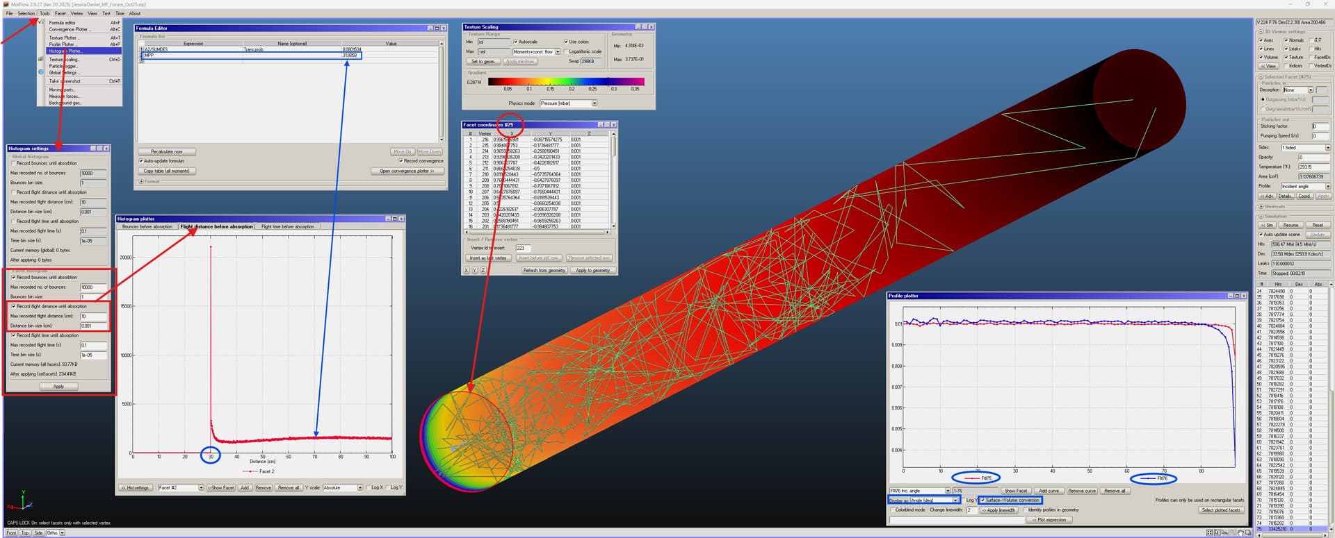
what you need is just to use the “histogram Plotter” features in the “Tools” menu, as shown in the screenshots.
I’ve created a 1 cm radius pipe with 72 side facets, and length adjusted to 30 cm so as to match you datum of a 8% transmission probability, with uniform desorption (from facet 1, the circle on the bottom left in the screenshots) and also uniform reflection along the side walls. The exit facet no.2, circle on the upper right, has sticking =1 like the inlet facet no.1.
I have created and added two facet, with opacity = 0 and “Incident angle” profile pull-down menu on the right of the screen, “Profile” field. They are facet no.75 and no. 76.
Facet no.75 is a copy of facet no.1 (the inlet for the gas), moved in the Z direction (axis of the pipe) by 0.001 cm with a normal vector pointing the other way around compared to facet no.2.
Facet no.76 is a copy of facet no.20, one of the rectangular side walls on the top (+Y direction) along the tube, moved down by dY=-0.001 cm, opacity=0 and “incident angle” profile, like facet no.75.
The two transparent facets thus created are used to visualise the impinging angular profiles, no.75 records the angle of EMISSION of the molecules from facet no.1 (minus a tiny fraction which escapes the 0.001 cm distance between facet no.2 and facet no.75, they cannot be coincident, a minor approximation, though). Facet no.76 records the UNIFORM REFLECTION of the molecules off facet no.20, one of the 72 around the cylinder.
They are plotted on the “Plotter profile” window on the bottom right. You can see that they are flat from 0 deg angle (i.e. angle of the molecular trajectories with respect to normal vector of the facet) up to almost 90 deg (i.e. parallel to the facet plane, and perpendicular to its normal vector).
The sudden drop near 90 deg is due to the fact that no molecular trace can cross the two facet at 90 deg, it is physically impossible with sticking=1 on facet no.1 and 2.
So, this confirms the correct implementation of this simple model as per your description.
Now let’s go the real question you ask: how to calculate the MPP, average length of the trajectories of the molecules reaching the exit, i.e. facet no.2.
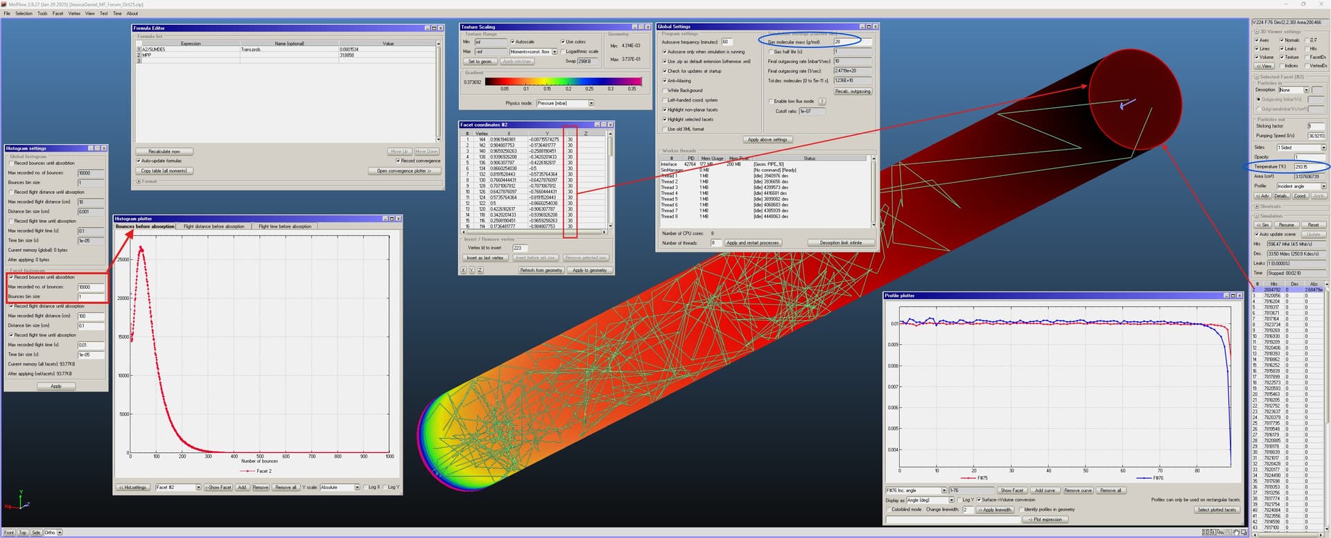
Using the “Histogram plotter” tool as indicated in the screenshots, you can calculate the number of bounce, length, and time taken to reach facet no.2. Simply select it and hit “ADD” for each of the quantities chosen, here 3 of them, “local” ones… “Facet histograms”, I mean, not “Global”… that would do something else.
I have circled and arrowed some quantities trying to explain how they are linked to the problem, should be self-explanatory… if not just ask and I’ll expand the explanation, no problem, now I can’t do it, sorry.
I include the Molflow+ zip file and the screenshots.
I only realised at the end that I should have chosen “Normalized” and NOT “Absolute” in the plots for the facet’s bounces, time, length… the “Absolute” shown in the screenshots varies as the number of generated molecules increases… while “Normalized” gives the probability distribution normalized to one, which is what you need to calculate the average time or length to reach facet no.2.
Cheers.
JessicaDaniel_MF_Forum_Oct25.zip (473.3 KB)