Pressure calculation on a tube (simple test case)

[guest_jmarc.duval (Jean-Marc Duval)]

Hi, and thanks for this great tool.

I have a very basic question about pressure calculation in a simple tube, based on the example in the “quick start power point presentation”. My problem is that the pressure plotted in Molflow does not match the analytical calculation from Pfeiffer (DP = Qpv / C and C = 12.1 D³/L, for air (M=28, T=294) so DP = 1/12.1 QpvL/D³)

I made the same calculation and plot for different diameters : the pressure should vary as 1/D³, whereas it my Molflow calculation it varies only as 1/D and the overall difference is proportional to the surface between formula and plotted pressure along a surface.

The interface for the plotting changed since the quickstart guide was edited (no more “normalize” box) so a misunderstanding of the pressure definition could explain that discrepancy. Also I checked the outgassing rate and in my try, I set it to a constant so it should not change with different diameters.

Any advice on how to solve that discrepancy (basic analytical calculations and Molflow)?

[rkerseva (Roberto Kersevan)]

Hello:

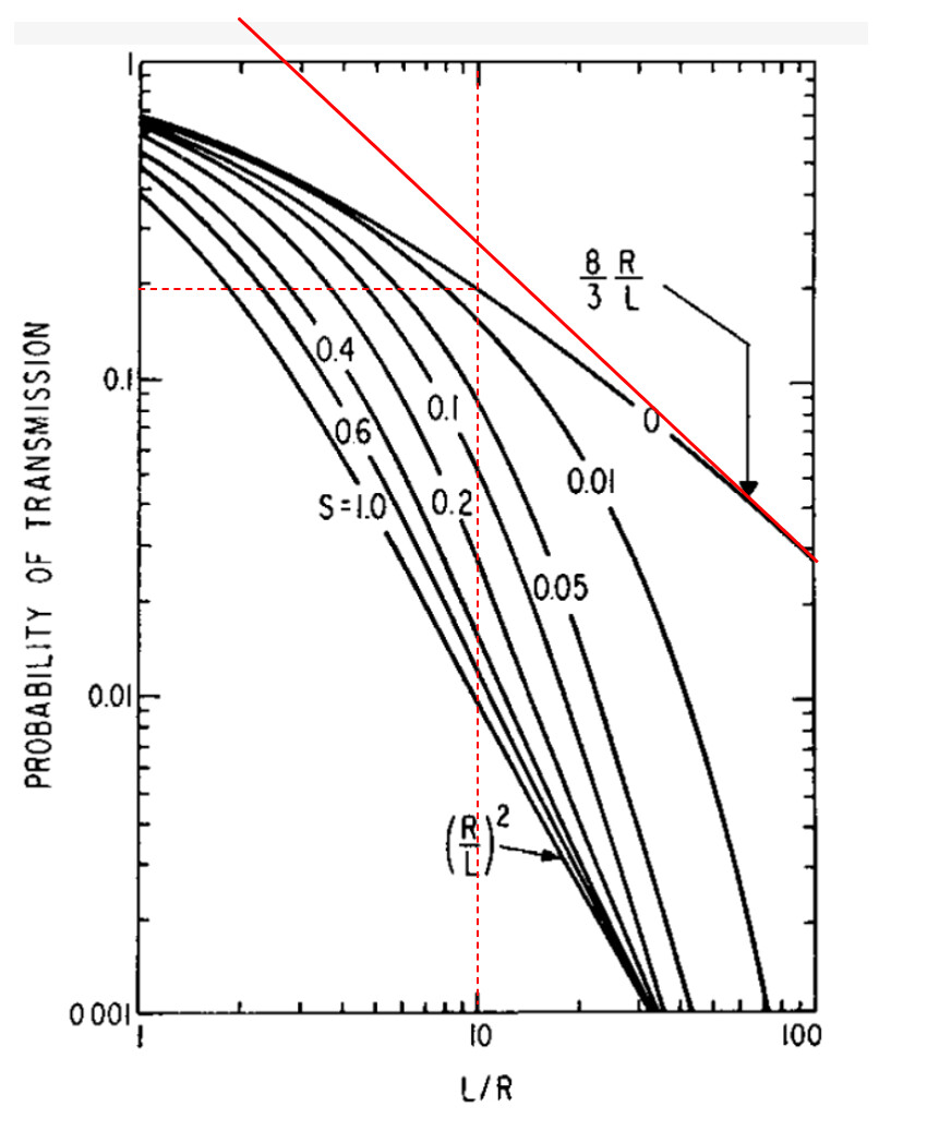
I am not sure I understand your problem: Molflow+ has been tested and validated extensively vs existing literature, in particular early papers on montecarlo simulations of transmission probabilities of tubes, like Smith and Lewin on Journal of Vacuum Science and Technology (see curve for the transmission probability vs L/R). This was the main subject of the 2009 paper, again on JVST A, by me and ESRF colleague Jean-Luc Pons.

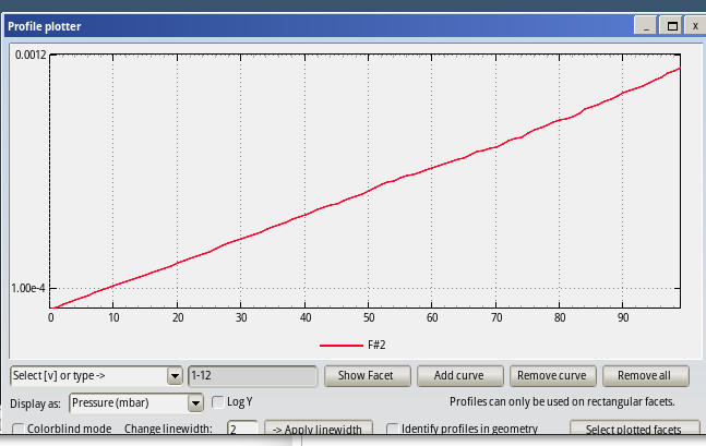
You didn’t include a model in your message, but if I quickly make a simple model of 2 cubes connected by a pipe of constant cross section (circular or other shape) and I calculate with Molflow+ the conductance of the pipe via C=Q/dP, with dP being the pressure difference inside the two cubes (I inject molecules in one and I pump in the other cube, as one would do in a lab to measure the conductance), I get results which deviates from your formula, see line 3 (your formula 12.1.D^3/L) and line 2 (C=Q/dP). P2 and P80 in formula 2 are the average pressure on the bottom facet of the two cubes. Ratio of the 2 values is about 1.36.

You say, rightly, that C should change as 1/D^3, and this is exactly what Molflow+ calculates: for a given diameter D C changes as D/L, and then there is the D^2 factor for the inlet area, since the transmission probability depends only on D/L. I do not see any discrepancy.

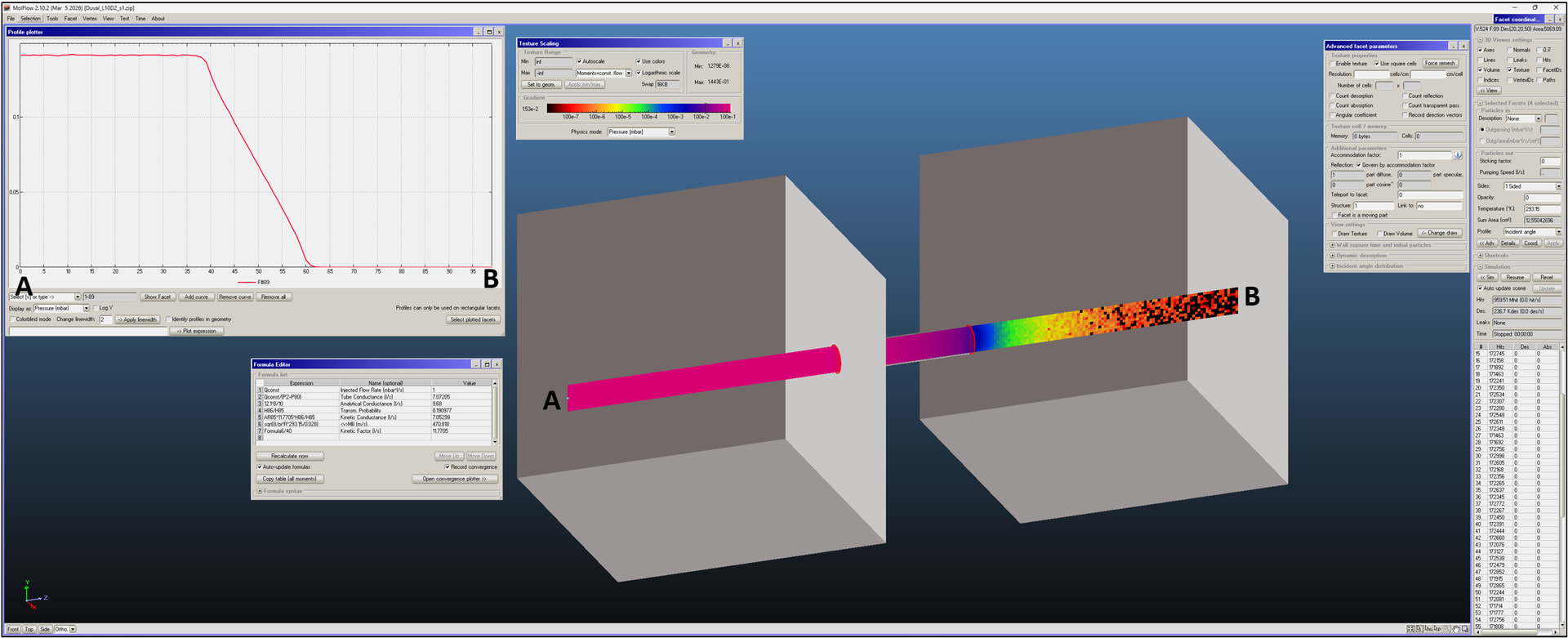
The model I attach has two 20-cm side cubes, connected by a L=10 cm, D=2 cm round tube.Molflow+ calculates P_tr (Transm. Prob.) of 0.191 (rounded), as per Smith&Lewin, see intersection of the two red lines.

The “kinetic” formula for the conductance (see “Formula editor” screenshot) is given by C=A*11.7705*P_tr, where 11.7705 is the l/s of a 1 cm2 opening for mass 28 gas at 20 C (293.15 K), a value given by the Maxwell-Boltzmann distribution integrated over a 1 cm2 opening, the /4 factor, with the MB average molecular velocity. See formula 6 and 7. The Kinetic Factor has a factor of 1/40 in the formula to go from m/s in the MB formula and Pa.m3/s (SI units) to the “Molflow+ units” cm and mbar.l/s (factor of 1000 for m3 to l/s, divided by 100 to go from m to cm. times 4).

The zip file attached has all 6 facets in the pumping cube (on the right in the view, see screenshot) with sticking=1, i.e. all molecules exiting the tube are pumped, and cannot go back to the tube, but if you change the sticking of these facets, or mimicking a real lab system you set sticking>0 only on one of them (the one with the physical pump) you get a similar value for the tube conductanc from formula 2.

See how in the model the conductance calculated via C=Q/dP and the kinetic conductance via the transmission probability match quite well, formula 2 vs formula 5.

So, it is clear that the often used analytical equation for the conductance is not valid here, since it gives a value of 9.68 l/s vs 7.07 of the Formula 2 or 7.05 of Formula 5 (1.36x higher).

The reason is that the 12.1.D^3/L formula is valid for LONG tubes only, i.e. where the transmission probability in the Smith&Lewin figure gets its asymptotic value of 8R/3L, in my model we are at L/R=10, still on the “bending” part of the curve labeled “0”.

The factor 1.36 is the difference (in terms of transmission probability) of the intersection point of the inclined solid red line and the vertical dotted line, with respect to the intersection of the two dotted lines on the Smith&Lewin figure.

If I make the tube longer, e.g. 30 cm instead of 10, I get a ratio of the conductance values calculated via the approximate formula line 3 and that on line 2 much smaller, i.e. in better agreement with each other. I Include the zip file too, it has L30 in the file name, the other one having L10.

If I make the tube 100 cm long I get almost a perfect match for the values in the approximated formula and the C=Q/dP, formula 3 and 2 (ratio 1.044, see file with L100 in the name).

The conclusion is that the formula C=12.1.D`3/L is valid only in the limit of LONG tubes, i.e. when L/R > 50 (where the curve with label “0” in the figure of Smith&Lewin coincides with a straight line with inclination -1 on the log-log scale.

That’s all, if not clear or further questions do not hesitate to write back, will be happy to expand on this important issue of vacuum science and technology.

R.

Duval_L30D2_s1.zip (118.5 KB)

Duval_L10D2_s1.zip (104.9 KB)

Duval_L100D2_s1.zip (150.1 KB)

[guest_jmarc.duval (Jean-Marc Duval)]

Dear Roberto,

Thanks for looking at my question, and sorry, it was not clear. Let me first assess that I’m convinced that Molflow is well validated. I’m pretty sure the mistake is on my part on the misunderstanding of the use of the interface.

So the simple_tube that I added to this message is simple : a tube (diameter 1 cm, length 1000 cm, 10 facets), with two opposite faces with a sticking factor of 1 and a desorption rate of 1e-2 for one of them.

When I calculate the different value I have:

Qpv = 0.01 mbar.l/s

C = 0.0121 l/s

DPexpected = 0.813 mbar

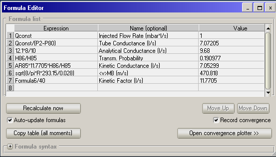
If I select one of the side face, add the profile “along face u” and then plot this face as “pressure” using the plotter, I’ve got more or less a linear profile along the tube, with a maximum value of 0.0012 mbar (see plot below)

The order of magnitude between these is not the same so I’m pretty sure I’m misunderstanding the plotting tool. I wonder if there is a “normalization” being done that I’m missing or if this is something else?

Best regards,

simple_tube.zip (71.8 KB)

[rkerseva (Roberto Kersevan)]

Hello again: in your model you have sticking=1 on both ends of the tube. That’s not correct, to apply the formula you must set S=1 only on one end, the one opposite to the gas inlet.

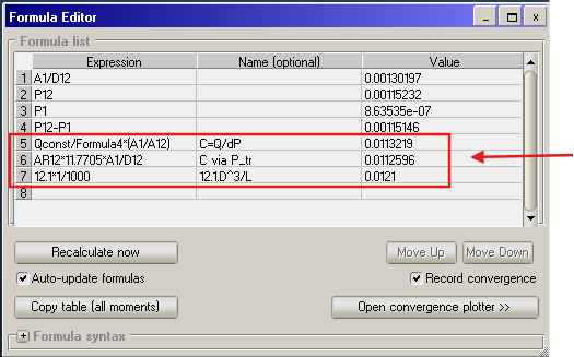
Otherwise, you should not use the C=Q/dP but C=Q*/dP, where Q*=Q x A1/A12, i.e. the ratio of the molecules pumped at the entrance divided by those pumped at the exit. In that case, the value of C is very similar to the expected one. It makes sense, because you want to “eliminate” all molecules which are pumped at the entrance, in effect only those reaching the exit count.

See file attached.

simple_tube_modRK.zip (94.5 KB)

Another thing you didn’t consider, is that pressure is NOT a scalar quantity, it is a tensor, meaning that its value depends on the orientation of the facet used to calculate it.

When you have sticking one on a facet, the pressure in its neighborhood is highly anisotropic: a pressure test facet placed immediately above it and pointing in the same direction (the normal vector) will “see” incoming molecules, but another test facet placed in the same position but with the normal vector reversed (pointing at the S=1 facet) will not see any molecule coming back, and therefore will register a pressure of zero.

The best way to use the simulation to calculate conductances via the C=Q/dP is a volume at the entrance where molecules are generated, a volume big enough that the molecules entering the tube have a cosine-like angular distribution (otherwise the transmission probability and the conductances are going to be different!), a volume with NO pumping, and then a second volume at the exit, where in principle you should add a pumping speed equal to the one of a real pump. In my previous examples I had set s=1 on all 6 20x20 cm2 facets, each having a pumping speed >4000 l/s, unrealistic under most reasonable assumptions (other than immerging the cube in liquid He), but still if you look into the file and look at the pressure calculated on the transparent circular facets at the entrance and exit of the tube (there are two pointing -Z and 2 pointing +z, facets no. 85 to 88) you can see that their pressures are not the same as the pressures calculated via the texture elements along the long facet… you can visualize those using the “Tools” “Texture plotter” command, after having selected it (facet # 89).

R.

[guest_jmarc.duval (Jean-Marc Duval)]

Thanks a lot for taking the time to explain Roberto, that helps a lot.

With this better understanding I will build a useful model for me from here.