Pumping manifold conductance

[e-nico911 (Edoardo Nicoletti)]

Hi,
last winter I started to study vacuum technology and now I’m working on to study a simple vacuum cavity (for RF test) and to design an appropriate pumping interface.
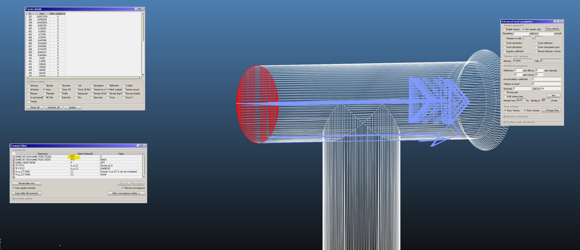
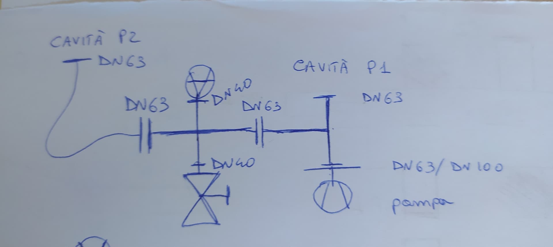
I designed a simple manifold made by two tee DN 63 according with the scheme in the figure attached. This solution allows me to pumpdown the cavity using one or two ports: one is connected directly to the cavity (P1); the second one using a pipe (P2).
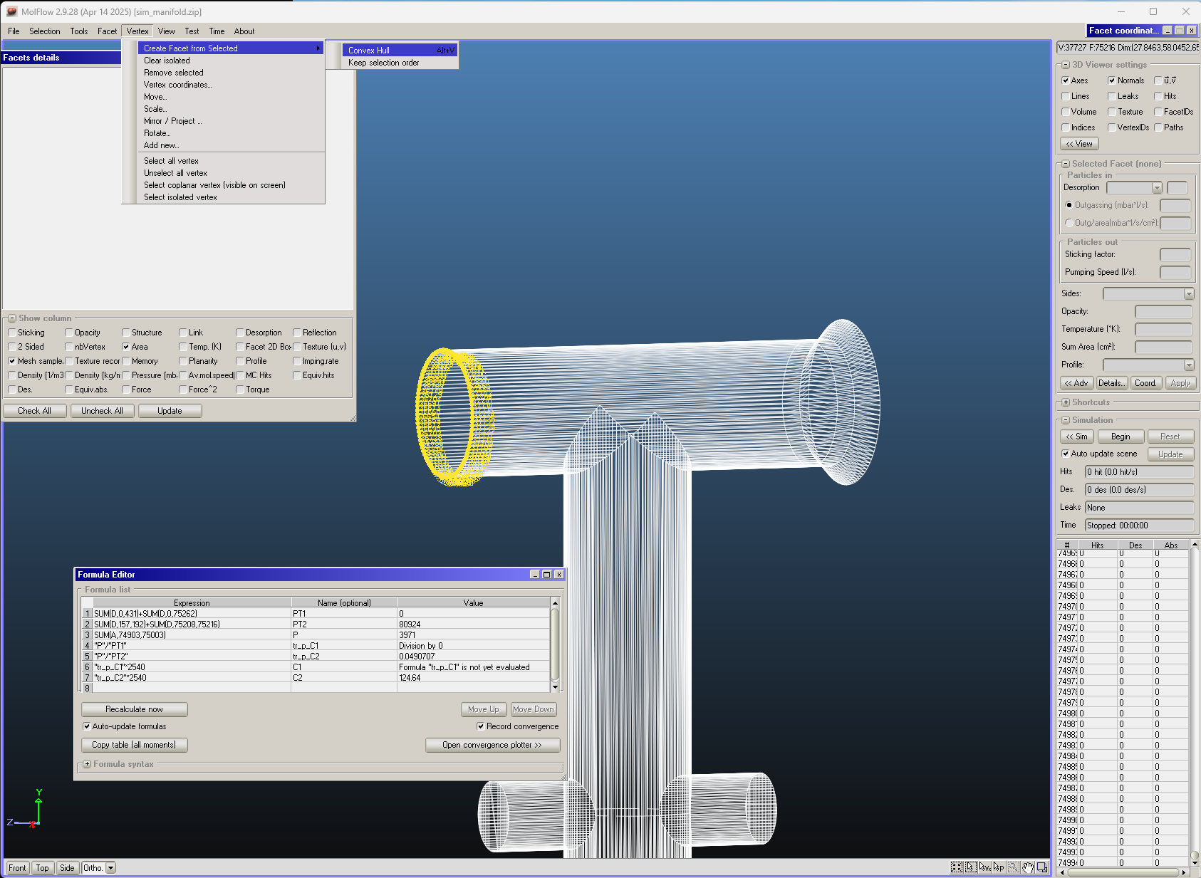
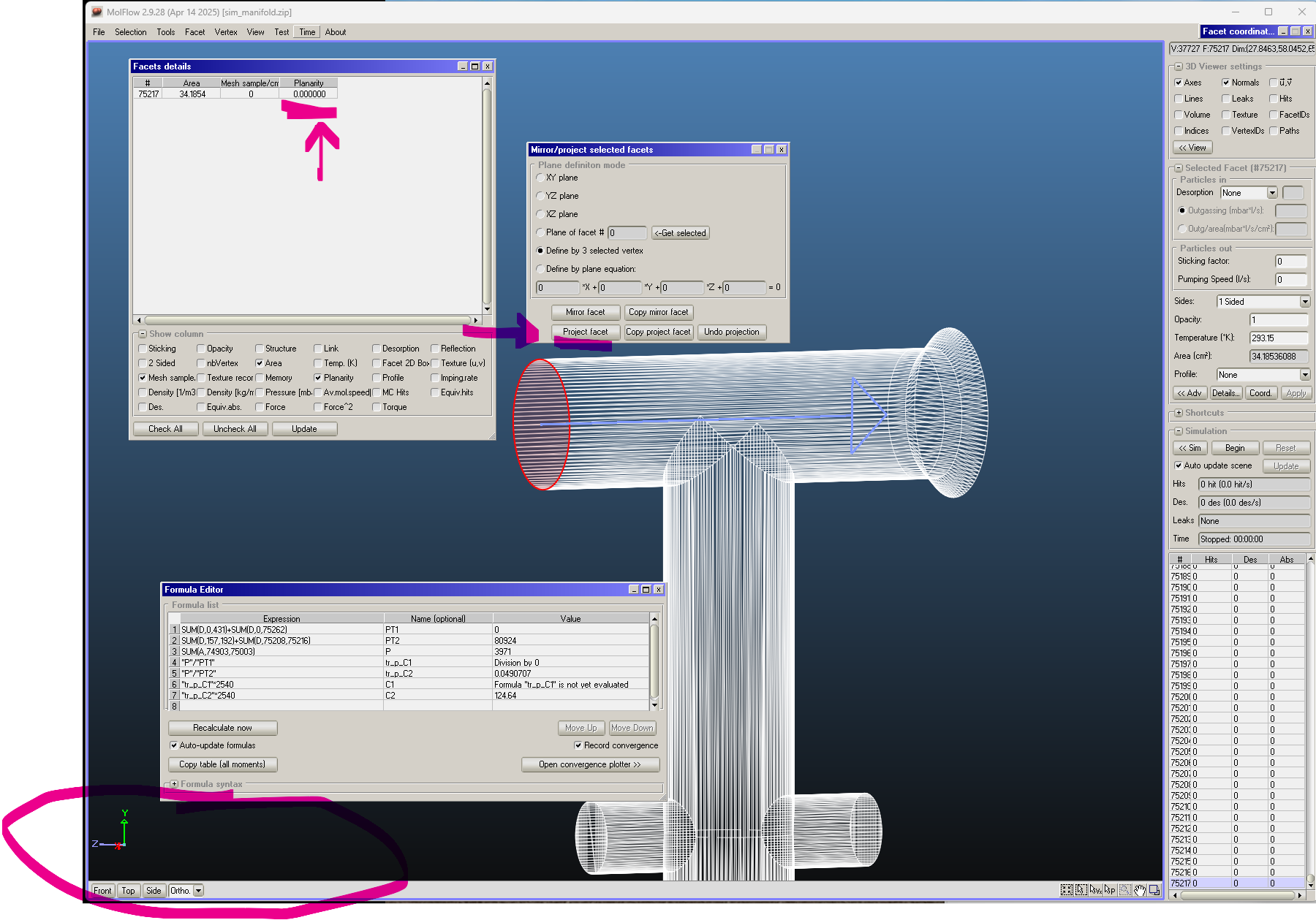
I made the 3D model of the entire volume but also of the pumping interface only. I made a simple calculation of the conductance of the manifold (direct port-pump; pipe port-pump) considering the hypotesys of short pipe and long pipe respectively. Now, I want to determine the conductance between the manifold, not only to confirm my calculation (I know that there is an error between simulation and analitical calculation - generally no more than 10%) but also to understand how to analyze a complex pumping interface (sometimes difficult to calculate) and, in this case, if it is a good choice.
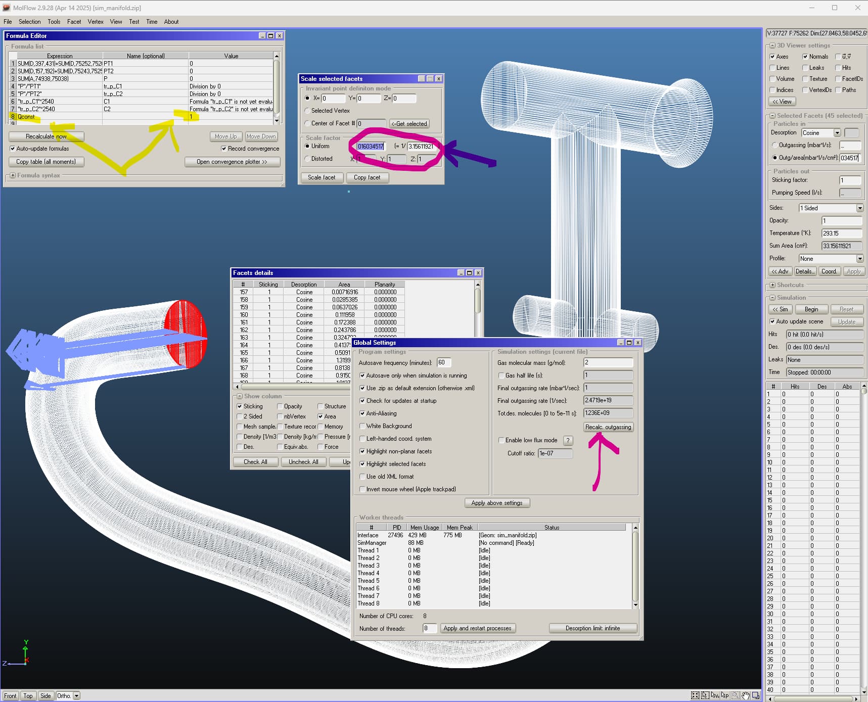
I prepared the simulation, as you can see in the file attached. I made this assumption:

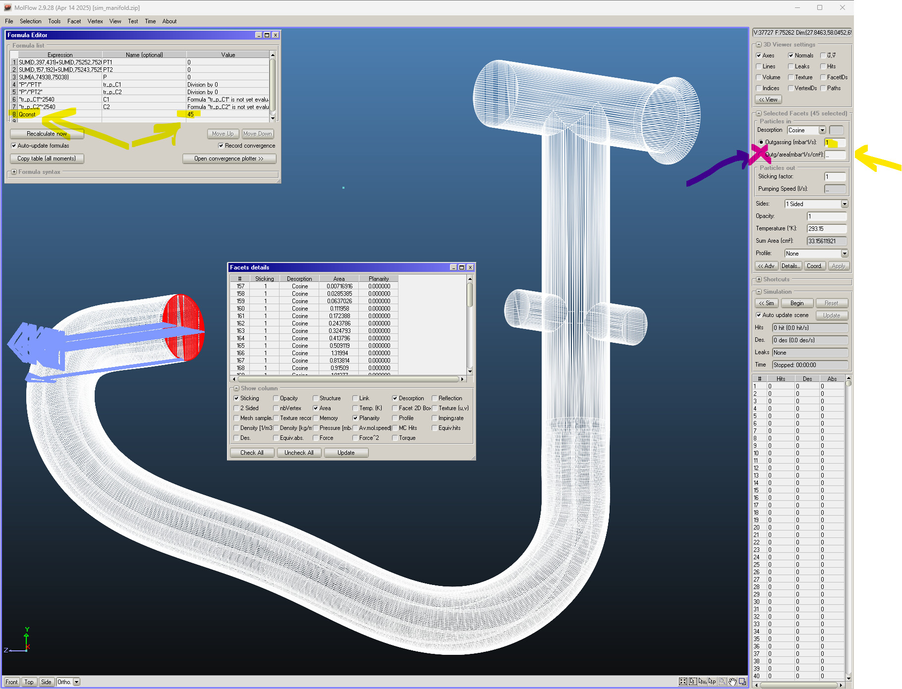
• pump port: sticking factor 1;
• cavity port 1 (direct): desorption cosine 1, sticking factor 1;
• cavity port 2 (pipe): desorption cosine 1, sticking factor 1;
• gas: hydrogen.

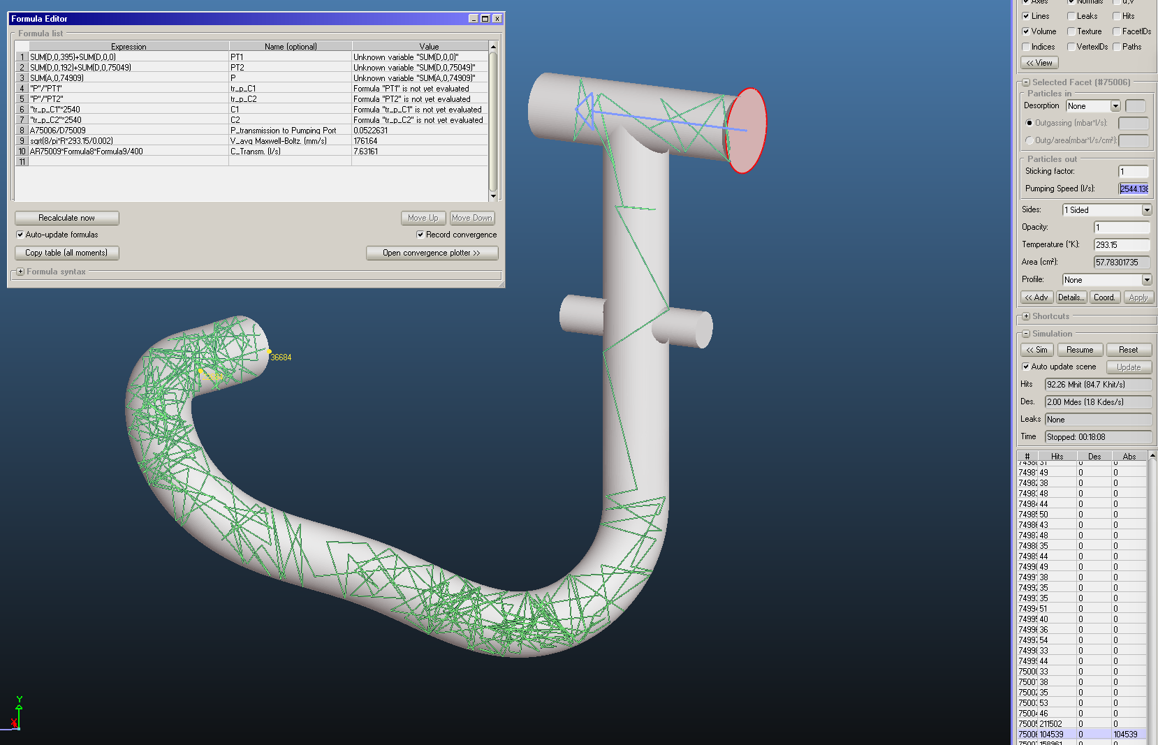
The transmission probability is calculated as usual: the ratio absorbe/desorbed considering the correct port for the desorption.

Now my the question are:

• if I set the desorption on both ports, the transmission probability is always the same for each coupler of ports. It is strange: maybe it is because the system is generating the same quantity of particle and at the end they are pumped away? It is correct, or I made some error or assumption? I still have some doubts.
• I considered one port at a time, and I found different conductance. This is correct but the for the short pipe I obtain a value double than the one calculated. I am not expecting some error Where I am going wrong?

sim_manifold.zip (4.2 MB)

Sorry for the long post. These are probably simple mistakes due to the fact that I am still inexperienced. But I think that is a good opportunity to learn.
Thanks a lot in advance for the help.

[rkerseva (Roberto Kersevan)]

Hello Edoardo, and welcome to the forum.
I looked at your file, and I have several points to raise, a few explanations, and some suggestions.

1. Your CAD-derived file has a very, extremely high accuracy, I mean the size of most of the facets is few HUNDREDS of a cm2. You may want to “relax” the parameter in the CAD program which generates the STL file. Anyway, even with this resolution, and 75262 facets, one could get the correct answers. I would have used the Molflow+ editing features, and build the model with at most a few 1000s facets, but that needs some “excercise” with the editor. Maybe matter for another post.

2. Ports’ geometry and definition: the 5 ports in the model, see figure, are defined by a total of 331 facets, when 5 would be enough. I will explain now, next point, how to do that.
   

   

3. I highlight here the facets of Cavity P1 (as per your sketch): according to your formula, this represents Cavity P1.
   First of all, you can save a lot of writing, plus if you re-arrange facets or delete some of them the formula doesn’t need to be redefined, by selecting those facets and SAVING them in a selection group… “Selection” menu, see figure…
   

   

You can then re-formulate the formula 1 simply as as SUM(D,S1) (if this group of facets is the first in the list of selected and saved facets), otherwise S2 if it’s the second one, and so on…
Then what you need to do to simply make one single facet for this port instead of the 46 facets of your model is to “collapse” them, by using the “collapse selected” command in the Facet menu. When you do that it generates one facet only BUT it is NON-PLANAR. This happens often when using CAD-derived STLs, especially when facets are not oriented parallel to one of the 3 axis (not 100% sure of this, just my impression).
In fact, COLLAPSE doesn’t work, unless one changes the coplanarity, collinearity etc parameters, which would generate one facet only but highly NON planar too, so not very useful.
So, the way to proceed is to DELETE these facets, and then select ALL vertices on the circular opening and creating a facet.

Once this is done, you can see that the facet is highlighted in pink, and there’s a warning message on the bottom left corner… “non-planar facets…”.
To correct this non-planarity you select 3 vertices on the circular facet and then use the “Facet” menu, “Mirror/project” command, with the “Define by 3 selected vertex” option… “PROJECT FACET” button.
Now you see that the facet is NOT highlighted in pink anymore, and its planarity is zero:

3. You should now re-do this operation for the other 4 ports: once you have done it, you-ll have 5 facets, appended at the end of the facets’ list (since they are newly created), and easy to address in a formula definition… no need to use a selection group as I mentioned earlier, simply their facet number.

4. Now let’s come to the vacuum physics part of your message, determining conductances and transmission probabilities.

5. The model you sent has the desorption at the end of the curved manifold: there’s a problem in the definition of the outgassing rate. You have selected “1” as the value, but this is the ABSOLUTE outgassing rate for EACH facet defining the port, independent of its area. I have added the Qconst pre-defined variable in the formula window (total outgassing for time-independent simulations), and you can see that it is 45 mbarl/s, since there are 45 facets each desorbing 1 mbar"l/s. This is not correct, you should define a uniform area-normalized outgassing rate, the SECOND option, in mbarl/s/cm2. If you want the total outgassing of the whole port to be 1, then you simply set as outgassing the RECIPROCAL of the total area of these facets (you can read the total area in the “Sum area )cm2)” filed, on the right pane, see figure here below.
   

   
   
   If you set the SPECIFIC outgassing of each of the 45 facets equal to 0.03016034517, then you get a Qconst=1. You can use the Facet scale option to quickly calculate reciprocals, just put one number in the first field and the second one will calculate the reciprocal automatically, see circled area on the figure. You also need to re-calculate the total outgassing in the “Tools” menu, “Global settings” window, button on the right, see pink arrow.
   
   

Transmission probability: on your model there is sticking=1 only on the pumping port, and on the desorbing facet, which on the model I attach to this is facet no. 75009. The pumping port is facet no. 75006.
I’ve defined a formula formula for the transmission probability, which is around 0.0515.
The next formula defines the TRANSMISSION CONDUCTANCE from Cavity P2 to the PUMP: it’s valid only for a uniform temperature T, because it uses the average molecular speed for H2, which depends on the square root of T, see formula line 9 (in m/s).
The transmission conductance is given by formula 10.
It is given by the product of the desorbing area, AR75009, times the transmission probability, Formula 8, times the kinetic MB factor for V_avg, Formula 9, and divided by 400.
Why this 400 factor at denominator? Because the formula would be 1/4 (comes from the integration in the MB distribution over a sphere), and the additional 100 factor comes from the fact that V_avg in Formula 9 is in m/s, but Molflow+ needs cm as units, so divide by 100.
Hope it is clear what I mean, if not I can explain further.
Notice how the INSTALLED pumping speed at the pumps’ port, which is 2544.14 l/s for H2, gets down to only 7.64 l/s, since the conductance will prevail (it’s a conductance limited system).
In this case the EFFECTIVE pumping speed is given by Seff=(1/Sinst+1/C)^-1=7.64 l/s.

5. If you need to calculate other transmission probabilities and conductances, and effective pumping speeds, then set the sticking of other ports =1.

Good luck, and do not hesitate to write back and ask for more details.

sim_manifold_modRK.zip (7.4 MB)

[e-nico911 (Edoardo Nicoletti)]

Hello Roberto,
thanks a lot for your welcome and the answer. Your explanations are clear, detailed and are truly precious.
I appreciate a lot the explanation on how to prepare the facets: I added it to my notes. I admit that I suspected some errors on those facets and I also was not sure about their setting (i.e. desorption rate) but now it is clear.
Considering the unitary setting for desorption and pumping (in this type of simulation), my settings were, let say, strange.
Regarding transmission conductance, the formulas and the results are clear. Now I know that I’ve used the correct formula and it is interesting that with these positions (area etc) I can obtain the effective pumping speed. I did not think about it.
But in this case or similar, where the conductance is so relevant, if I want to study the manifold can we set the simulation with “real” pumping speed? In any case, I noticed, we have to consider each port at a time.
Last question (more conceptual, sorry). In your opinion, how can be useful or convenient to calculate analytically the conductance in these cases? I have the habit to do it and sometimes even not perform any simulation. Probably it is more convenient to perform a simulation with the complete system, right?
I will spend some time to explore better the software and how to prepare the model and obviously delve further into the vacuum theory.
Thanks again!

[rkerseva (Roberto Kersevan)]

Hi Edoardo:
you can certainly set the simulation with the real pumping/sticking coefficient at the pumps’ location, but that will not change the result.
If you really want to grasp the effect of conductance of the different parts making up your model, and possibly try to remove or optimize any eventual limitation point in it, then I suggest that you add a transparent facet (opacity=0), 2sided, along the vacuum system. Unfortunately the geometry of your model, with those twisted parts bending in different direction (and without me knowing the radius of curvature and angles of rotation of the various segments) prevents me from showing to you how to do it along the whole model… but I can add a few facets here and there placed along the axis of the various parts, and calculate the effective pumping speed at EACH of those points.
So, I have added 2 facets, as described: one horizontally into the pump, the second one vertically down from the “T” where the pump is attached.
The pump i still at s=1, i.e. 2544 l/s for H2 at 20 C. You can change that later, and re-run the program.

You can see the two pressure profiles along the two transparent facets: the orientation depends from the u and v axis (top right corner) and the choice of the pressure profile (pane on the right, either along u or along v). The pressure plotter shows the calculated pressure for each of 100 slices of equal width along the rectangula facet, slices cut along the u axis, in this case. The horizontal scale of the pressure plotter is always 100 units, no reference to the ACTUAL length of the rectangular test pressure facet.
Red curve is the horizontal test facet, left to right, the blue one is the vertical one, bottom to top. If you click with the mouse on any of the two lines you’ll get the value of the pressure along the corresponding slice. You can also select, copy and then paste (in e.g. Excel) all of the 100 values, simply with the mouse on top of the vertical scale numbers and right-click with the mouse, and then select “Copy to clipboard”. Maybe you knew alread all this, anyways…

I also added textures on the two transparent facets, with texture size 1x1 cm2. See highlighted parts on the second figure here below:

I’ve set 1x1 cm2 texture elements, as highlighted in the “Advanced facet parameters” window.
If you open the “Texture plotter”, in the facet menu like the profile plotter, you can click with the mouse on each of the pressure values, or select rows, columns, rectangular blocks of cells, and then copy/paste them (again, right button of the mouse).
I have added in the screenshot 2 formulae:

No. 11 is the pumping speed of the facet with sticking 1. Notice the factor 40 in the denominator, not 400 as I mentioned in the previous message… 40 is correct, 400 is 10x too big, sorry, my mistake, please keep it into account for the other message tool.

The last formula, no.12, is simply one test of how to calculate the local effective pumping speed: since the total outgassing is 1, the S=Q/P formula gives me S (in this case Seffective at that point, simply computing the reciprocal of the pressure. If Q is not one you should substitute the 1 in the formula with Qconst (the pre-defined variable). The value of 767.413 l/s for Seff is valid at the square texture highlighted when selected clicking on the table:

If you want to have the Seff for the real case, when the pump has not sticking=1 but, say,only 0.1179181, corresponding to 300 l/s, then you set sticking to that value (or write 300 in the pumping speed field and Molflow+ will automatically calculate the corresponding sticking) and re-run the simulation.
After a few minutes, I get this:

Seff is now only ~228 l/s, which makes sense because the place where I’m looking at is not far from the pump, and therefore the Seff there must be of the same order of Sinst.

I attach the file for the latter case of Sinst=300 l/s.

Good luck!

sim_manifold_modRK2_300ls.zip (7.3 MB)

[e-nico911 (Edoardo Nicoletti)]

Hi Roberto,
first of all, sorry for this late reply.
Thanks for your suggestion. The explanation is perfect (don’t worry if is not complete). This idea is very interesting. I will try to replicate and extend my study. Thanks a lot!