Subject: Clarification on how Molflow relates density, pressure, and impingement rate

[100013312 (Saurabh Kumar Singh)]

Hello everyone,

I am trying to understand how the different physical quantities in Molflow are interconnected—specifically density, pressure, impingement rate, and speed. I am finding inconsistencies that I cannot fully explain.

If I manually try to compute the impingement rate using:

flux = density × speed

the result does not match the impingement-rate plot shown by Molflow.

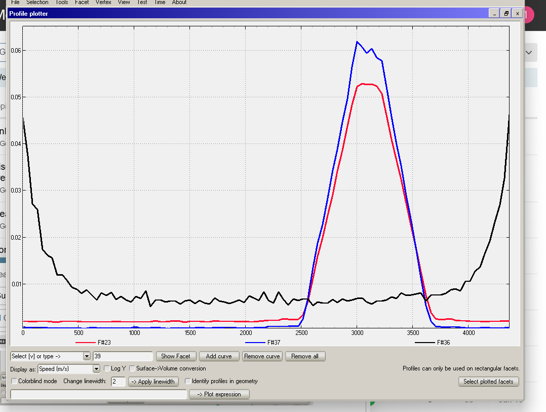
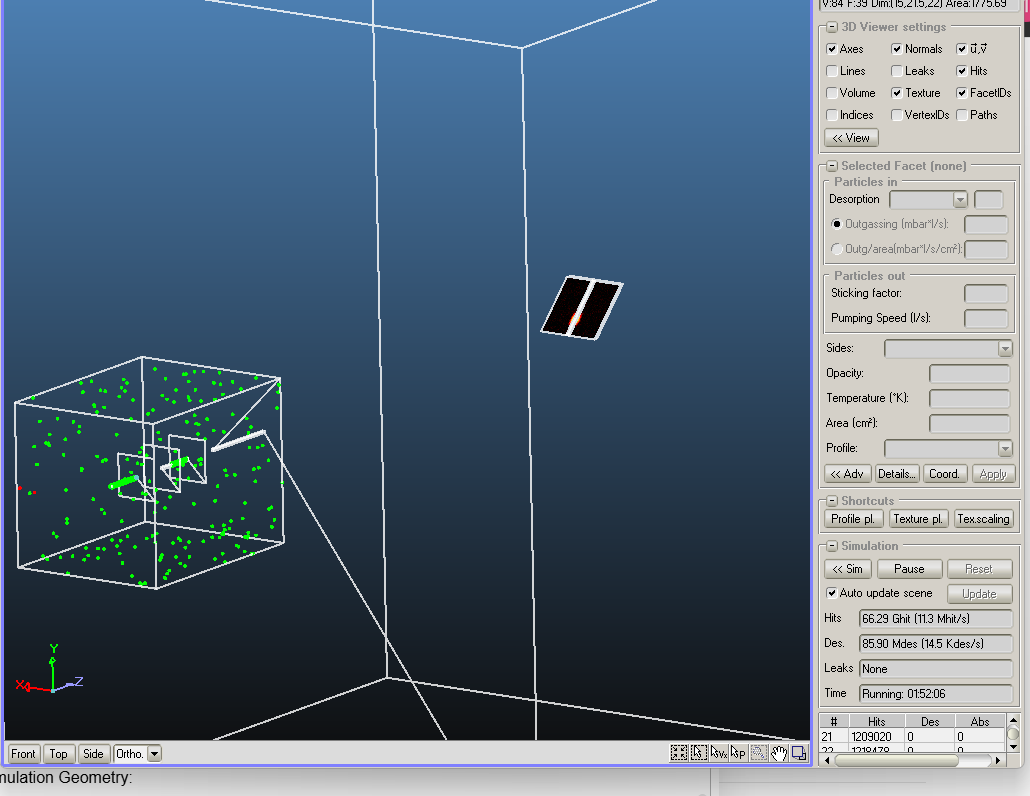
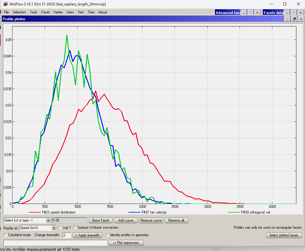
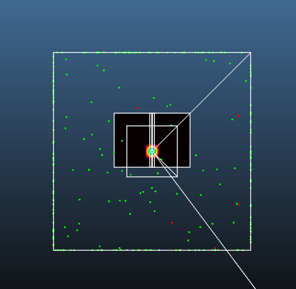
In my simulation the beam divergence is extremely narrow (≈7 mrad), and I am using the molecular speed directly from the Molflow “calculated profile” for our beam at the target surface. Our physical setup uses a two-stage cascaded capillary tube to obtain a highly collimated helium beam. In Molflow, the beam looks correct—collimated and narrow—but the numerical outputs confuse me.

My questions are:

1. Which speed does Molflow internally use for converting density → flux and density → pressure?
   (thermal speed, injected beam speed, or something else?)

2. How exactly does Molflow compute pressure from density?

3. Why does the impingement rate shown in the facet results not match the value obtained from “density × speed,” even for a nearly parallel beam with very small divergence?

4. Do the angular distribution and Monte-Carlo weighting influence the averaged speed that Molflow uses?

A brief clarification on these relationships would really help me correctly interpret the simulation outputs.

Thank you very much.

Best regards,
Saurabh

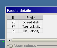
Output beam profile at target surface (in density):

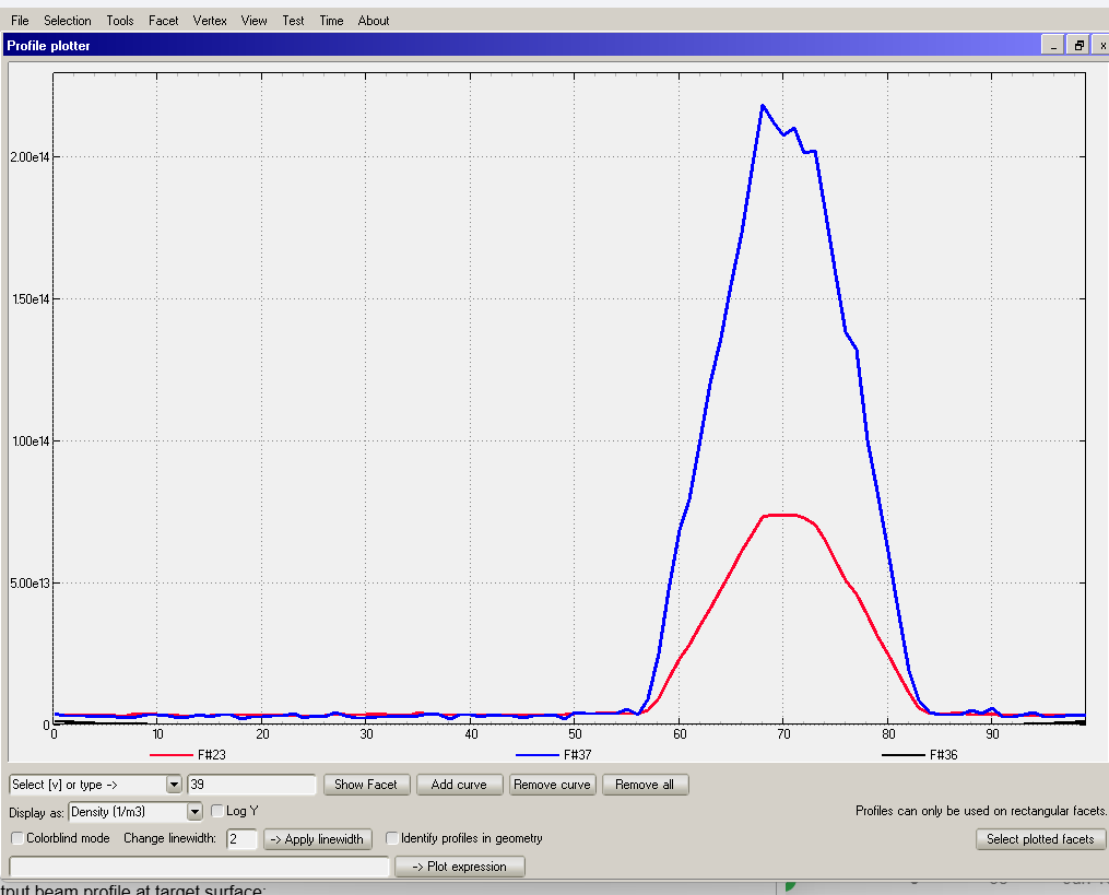
Output beam profile at target surface (in pressure unit):

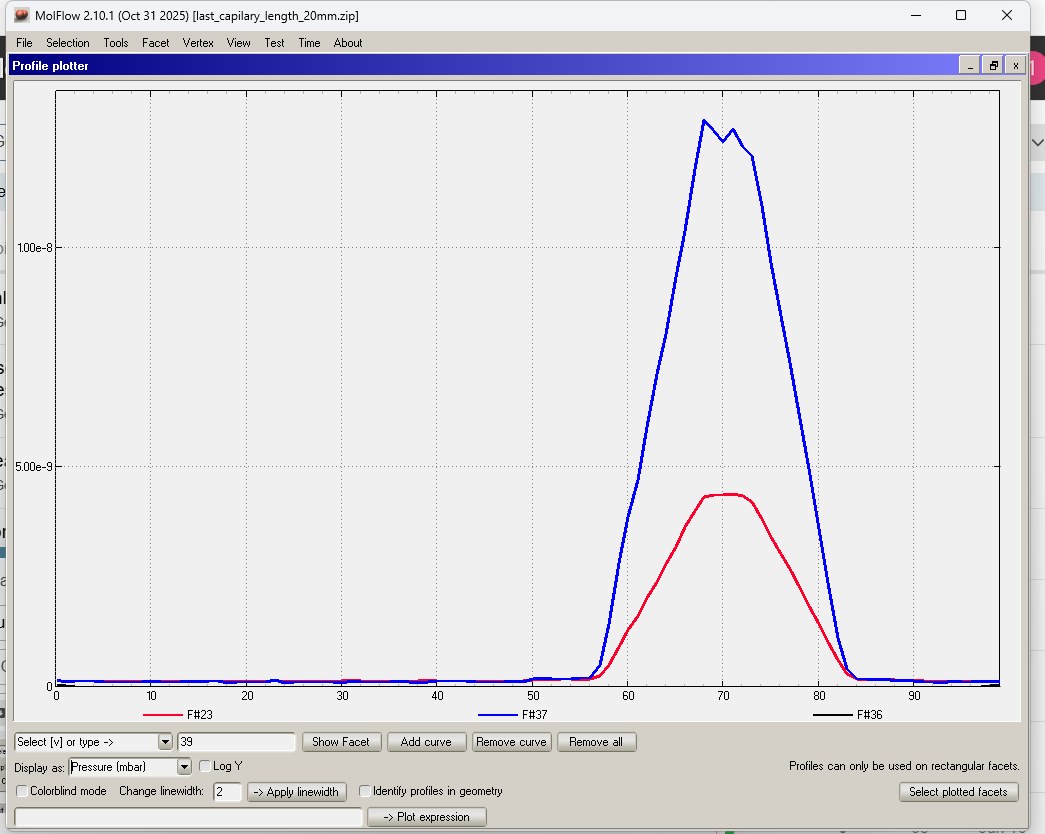
Output beam profile at target surface (in m/s, speed):

[maarton (Marton Ady)]

Dear Saurabh,

Physical quantity calculation is documented in detail in the manual, section 2.8:

The algorithm behind MolFlow+ - MolFlow / SynRad documentation

Notably, MolFlow does not convert between impingement rate (flux), density and pressure, since that would assume isotropy, which is not true in most cases, and certainly not in case of a molecular beam.

If you read this and some questions remain, please let us know. In case of a discrepancy, please attach a minimal example with the expected results and what you get instead.

I also think your last screenshot is wrong, you need to set up a speed profile on the facet, not just switch display mode to speed in the plotter.

Thank you, Marton

[100013312 (Saurabh Kumar Singh)]

@maarton

Dear Saurabh,

Physical quantity calculation is documented in detail in the manual, section 2.8:

The algorithm behind MolFlow+ - MolFlow / SynRad documentation

Notably, MolFlow does not convert between impingement rate (flux), density and pressure, since that would assume isotropy, which is not true in most cases, and certainly not in case of a molecular beam.

If you read this and some questions remain, please let us know. In case of a discrepancy, please attach a minimal example with the expected results and what you get instead.

Thank you, Marton

Dear Marton,

Thank you for your response and for directing me to section 2.8 of the documentation. I now have a clearer understanding of how MolFlow handles these calculations.

If I have any further questions, I’ll reach out with a minimal example.

Best regards,
Saurabh

[100013312 (Saurabh Kumar Singh)]

Hi Maarton,

Thank you for pointing out the importance of applying the speed distribution measurements for the facets.

Before asking my questions, I would like to briefly explain my simulation setup, which might help clarify my confusion.

I am simulating the behavior of a cascaded capillary tube (0.5 mm diameter, 50 mm length) designed to produce a molecular beam at the end of the capillary. We have set the parameters to operate in the molecular flow regime, and I am measuring the beam profile at 120 mm from the final end of the capillary.

I have measured three velocity profiles on the facet: speed distribution, orthogonal velocity, and tangential velocity. I have attached the screenshot of these velocity measurements for your reference.

As I observe, the beam coming from the capillary appears highly collimated with a 7 mrad divergence (final beam size of 1.8 mm at the screen). However, the transverse velocity profile appears very broad, which seems to contradict the collimation of the beam.

My confusion lies in this: If the transverse velocity is broad, how can the beam divergence be so narrow? For instance, if the mean velocity is 1 mm/µs, then at a distance of 120 mm, the transverse velocity should be quite small to give such a narrow final beam size.

Also, I’m wondering if tangential velocity and transverse velocity refer to the same thing in the context of this simulation. I couldn’t find much information about the calculation of transverse velocity in the documentation.

Could you please help clarify this apparent contradiction?

Thank you for your time and assistance.

Best regards,
Saurabh

Simulation Geometry:

Velocity profile measurement at 120 mm:

[rkerseva (Roberto Kersevan)]

Hello,

my first guess, if you don’t mind the intrusion:

The geometric collimation will not “collimate” the velocity profile. It will always be a Maxwell-Boltzmann-like distribution. You can reduce the width of the distribution by cooling the last stage of the collimators/capillaries, but that will also cool down the longitudinal velocity component.

You could collimate the tranverse velocity distribution by selecting only molecules of a given velocity, e.g. putting two rotating discs with an angular opening that spin and select only molecules leaving the last capillary at a chosen velocity, like a monochromator.In this case the transverse velocity vector would be the longitudinal one times the tangent of the average divergence angle, geometrically, with a small delta_V given by the angular width (times the spinning frequency) of the rotating discs. I have seen a similar set-up in a paper in JVST A or B, but can’t remember the exact reference, sorry. In this case you would have to run a time-dependent simulation, although the rotating discs with slots would need some thinking…

[maarton (Marton Ady)]

Dear Saurabh,

Can you plase attach the simulation file here?

Thank you, Marton

[100013312 (Saurabh Kumar Singh)]

Dear Marton,

Please find attached the simulation file as well as a research article we published a few years ago, which uses the same principles. I believe it might be helpful in understanding the scenario and simulation setup in greater detail.

Best regards,
Saurabh

last_capilary_length_20mm.zip (318.6 KB)

A compact and highly collimated atomic_molecular beam.pdf (6.3 MB)

[100013312 (Saurabh Kumar Singh)]

Hello,

Thank you for your input; I fully agree that the velocity distribution along the propagation direction of the beam will follow the Maxwell-Boltzmann distribution, as expected.

However, my concern lies with the transverse velocity distribution. Since we used a cascaded capillary setup instead of a single capillary, the design should theoretically allow us to filter the x and y components of the velocity, permitting only the z component to pass through the end of the capillary. We actually tested this approach a few years ago, and I’ve attached the relevant paper for your reference.

The issue I’m encountering is that my experimental results are not aligning with the simulated transverse velocity distribution. Based on our past experience, I was expecting the transverse velocity to be minimized in a highly collimated beam, but that doesn’t seem to be the case here.

A compact and highly collimated atomic_molecular beam.pdf (6.3 MB)

Best regards,
Saurabh

[maarton (Marton Ady)]

Hello Saurabh,

As in my first message:

“I also think your last screenshot is wrong, you need to set up a speed profile on the facet, not just switch display mode to speed in the plotter.”

Your geometry has no angular profiles.

[100013312 (Saurabh Kumar Singh)]

Hello Marton,

Apologies, I mistakenly sent you the wrong file. The file I shared was the pressure profile measurement, not the velocity profile that I intended to send.

I had changed the parameters to select the velocity profile at specific facets (#23, #37 and #39), but I think it wasn’t autosaved properly, and I ended up sending you the outdated file.

Please give me a few moments, and I’ll send you the correct version shortly.

Best,

Saurabh

[100013312 (Saurabh Kumar Singh)]

please find the corrected file attached.

velocity_profile_meas_cascaded_capillary.zip (100.7 KB)

[rkerseva (Roberto Kersevan)]

Hello:

I forgot to add a reference to a paper using Molflow+ and modeling multiple capillaries in series, here it is:

Cascaded collimator for atomic beams traveling in planar silicon devices, C. Li et al., Nature Communications (2019)10:1831, Cascaded collimator for atomic beams traveling in planar silicon devices | Nature Communications

[maarton (Marton Ady)]

What do you expect and what do you get instead? For me the profiles look as expected on a facet with 45-degree beam incidence.

[100013312 (Saurabh Kumar Singh)]

Thanks for your reply.

I would expect a narrow transverse-velocity distribution for a highly collimated beam. While the peak velocity in the simulation matches the expected (v_orth = v cos (theta) scaling for (theta = 45-deg), the transverse-velocity distribution appears much broader than expected.

If this broad distribution is correct, it’s unclear how such a highly collimated beam could be produced. As you can see in the attached reference paper, the transverse velocity is almost negligible.

[maarton (Marton Ady)]

If the beam incidence is at 45 deg, the two components v_ort=v_tan are equal (1/sqrt2*v_in) by definition.

You should set these profiles on facets perpendicular to the beam and you’ll get what you expect, narrow tangential and wide orthogonal profile. I just checked.

[100013312 (Saurabh Kumar Singh)]

Thanks for the clarification! After changing the facet to perpendicular, I’m now getting the expected results. Your explanation about the tangential and orthogonal components at 45° was really helpful.

Appreciate your help!