Hello Steven and happy that the registration went fine in the end 
I am looking to run a long time scale simulation (approx 30 sec real world time). Unlike simulations we’ve previously done in molflow, we want to start this simulation such that at t=0, the system is in a predetermined condition (pressure, temperature etc). How is best to do this?
For time-dependent basics, there’s an article, a tutorial and a video to get started. 30seconds is not extremely long, if your geometry’s size is typical (with a few cm mean free path).
Since Molflow is an event-driven simulator, only interactions with walls are supported, there is no “state” of the volume, just the walls. For that reason, you have to precondition the system, which is typically achieved through a time-dependent outgassing (a short pulse inserting all the required particles), then a time-dependent opacity facet that acts as a valve on the buffer volume (when system state equalizes to the desired pressure, you can open the valve by setting its opacity to 0 through a time-dependent parameter).
Note that while you have to find the equalizing time by trial and error, as all ultra-high vacuum systems are linear, you can calculate the required gas particles to insert.
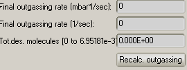
You have some diagnostics tools for time-dep. simulations in the Global Settings window, showing you the total number of particles inserted:
Finally, temperature parameter is currently not time-dependent, though we plan to make it so.
Additionally, some simulations we’ve done have been generating results that are confusing. Does it stand to reasoning that a surface or object made of stainless steel would offgas less at a higher temperature (say from 20* c to 50*c)?
I think the problem comes from the understanding of how Molflow converts outgassing rates to actual number of particles. (The pressure is calculated at an elementary level, taking into account the number of physical particles hitting an area per second, and their mass and speed, see details here in section 2.8) Molflow does not simulate the material’s (typically) increased outgassing when temperature increases, see my answer in this topic. If you enter a given numerical outgassing value, like 1E-3 mbar.l/s, then later change the facet temperature, the outgassing will stay the same (1E-3).
The reason that you’ll have a lower pressure in this example is because of the following:
- You’ll actually insert less particles in the system. From the ideal gas equation,
pV=NkT we can get the differential form Q=d(pV)/dt=dN/dt*kT where the left side is outgassing (in Pa*m3/sec SI units). If you keep the left side constant, but increase the temperature on the right side, the outgassing expressed in particles/second decreases: dN/dt=Q/(kT)
- Now you have less particles in your system. It is true that their speed is higher:
v_RMS=sqrt(8*PI*R*T/m), however the decreased particle count (~1/T) outweighs the increased speed (~sqrt(T)) resulting in a lower pressure
Since temperature-dependent outgassing is a material-dependent quantity, you have to manually enter the higher outgassing value for the increased temperature.
Hope I explained clear, get back if need concrete help,
Good luck, Marton