Unexpected absorbed SR photon distribution in Synrad+

[andrii]

Dear Synrad+ experts,

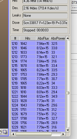
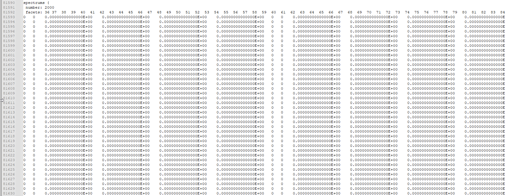
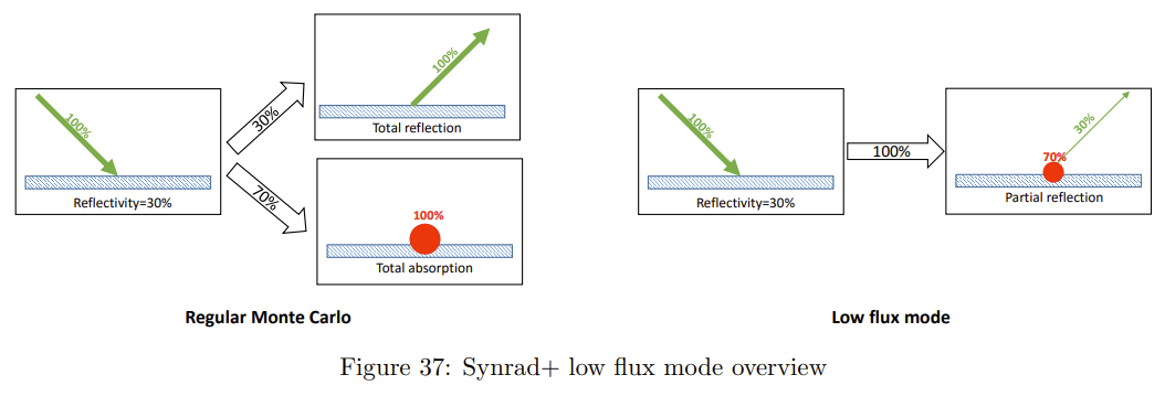
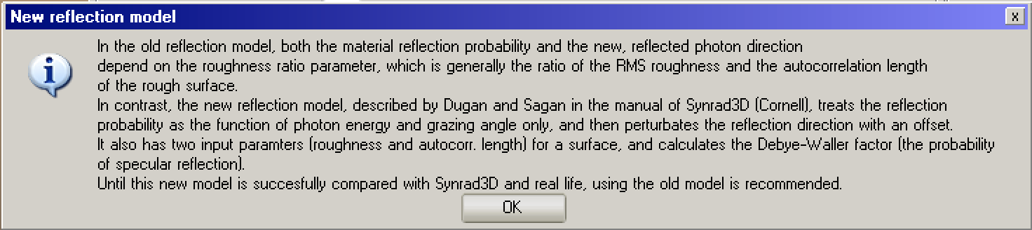
I’m working on the synchrotron radiation (SR) background simulation for one of the HEP experiments. I simulate the SR background in a particle detector from the electron accelerator. Initially, I planned to use Synrad+ for this task, but the problem is that Synrad+ cannot simultaneously store SR photon data (flux, energy, position, and direction) for all facets. And since we have about 30k facets, it is almost impossible to store the information one by one (it takes ages). Therefore, I decided to switch to Geant4, implementing SR photon reflection there using Synrad+ scattering probability tables (e.g., 02-Copper.csv), while reflection angles (theta and phi of the specular reflection) are smeared according to the following rule: thetaOffset=atan(sigmaRatio*tan(PI*(rnd()-0.5))); and phiOffset=atan(sigmaRatio*tan(PI*(rnd()-0.5))); from here.

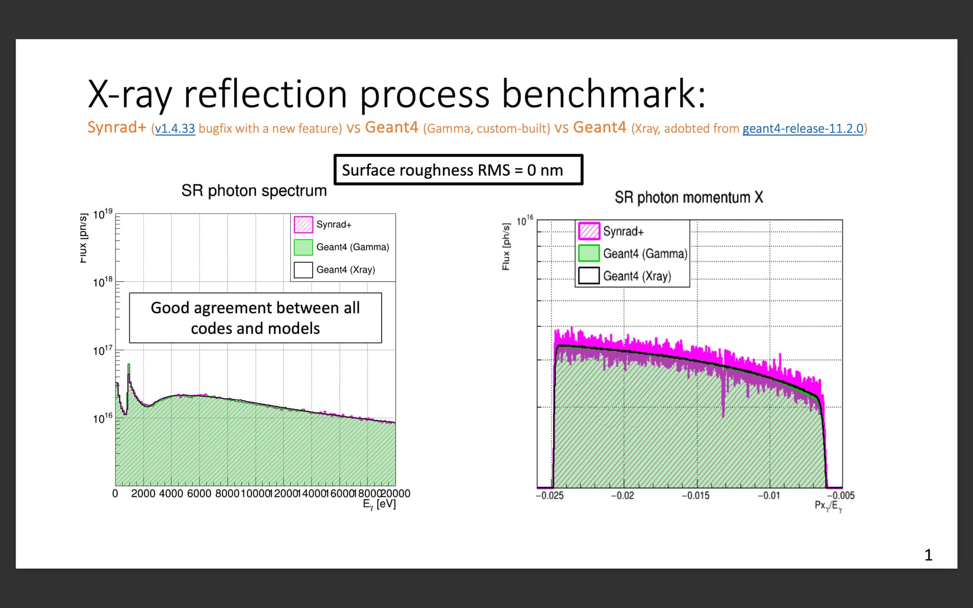
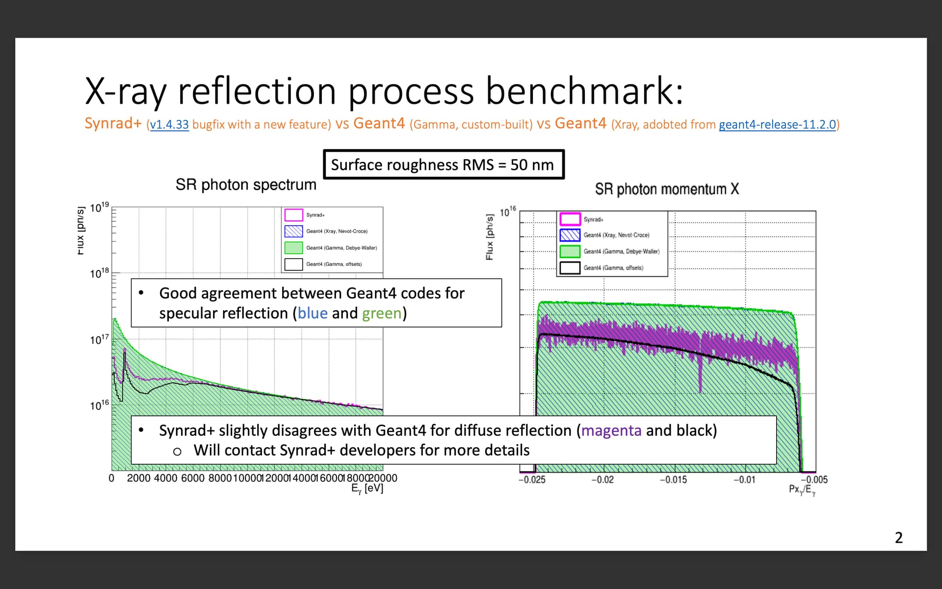
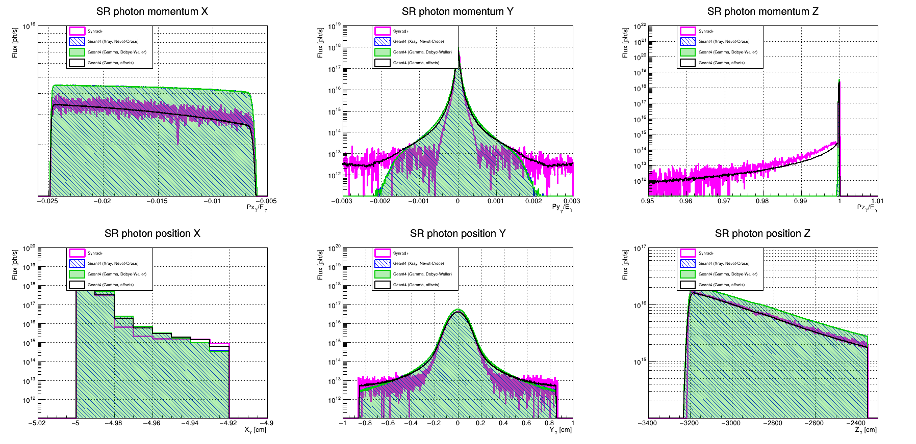
Before using my Geant4 code, I performed a benchmark in order to find possible bugs and improve the code. A concise summary can be found here.

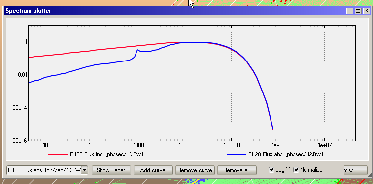
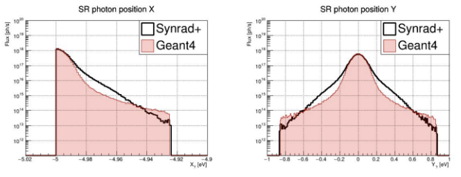
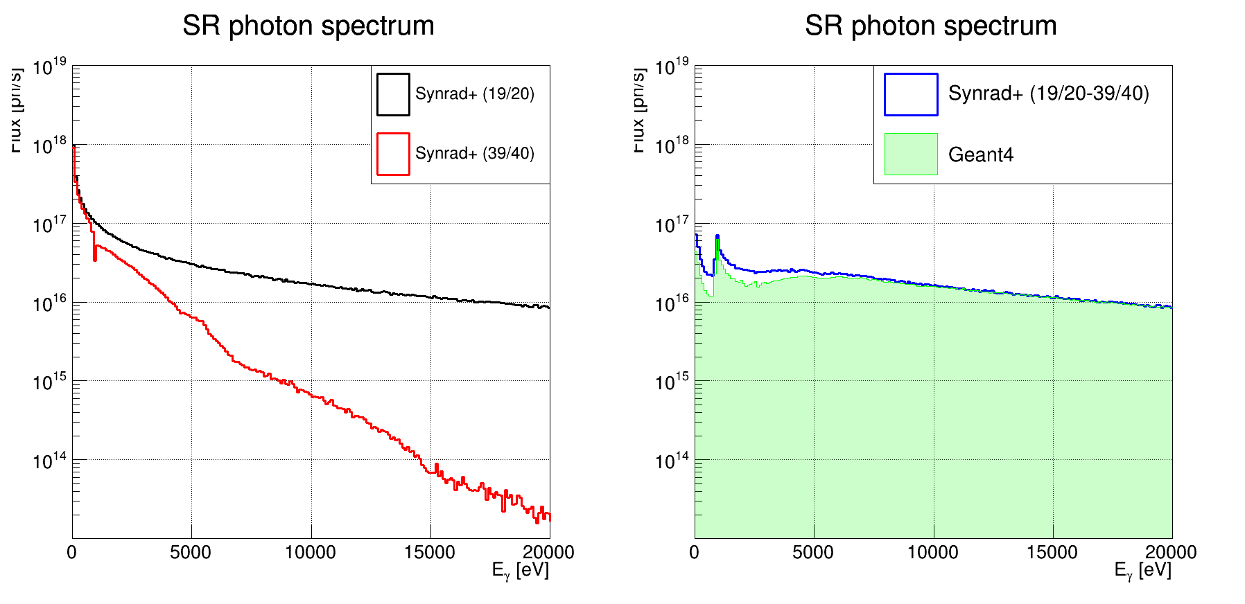
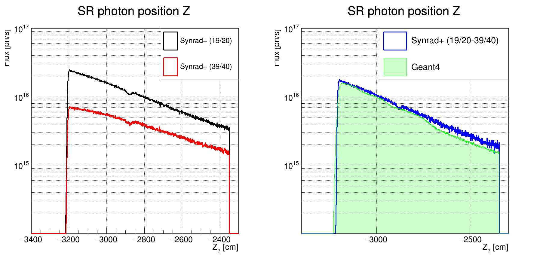
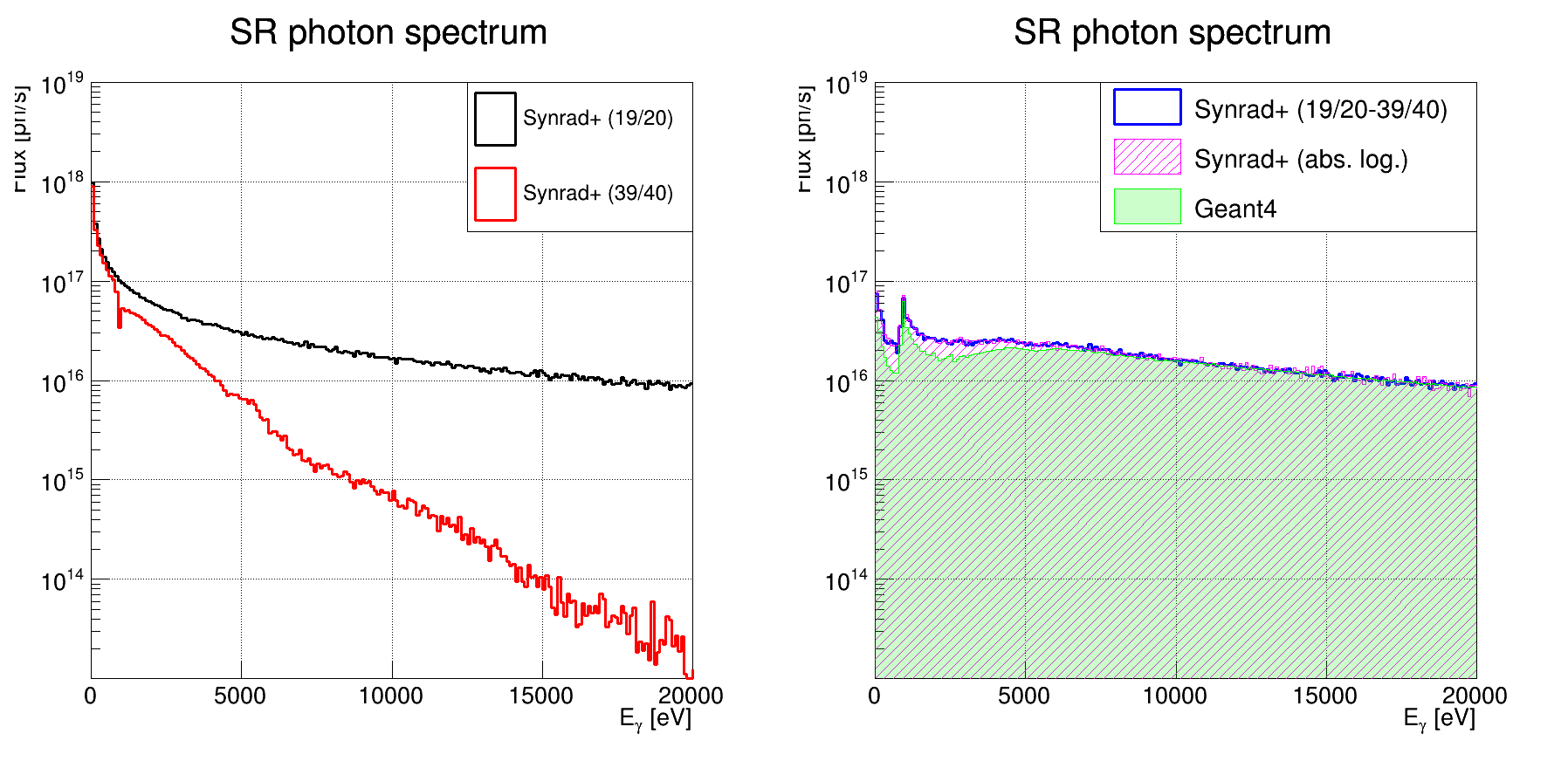
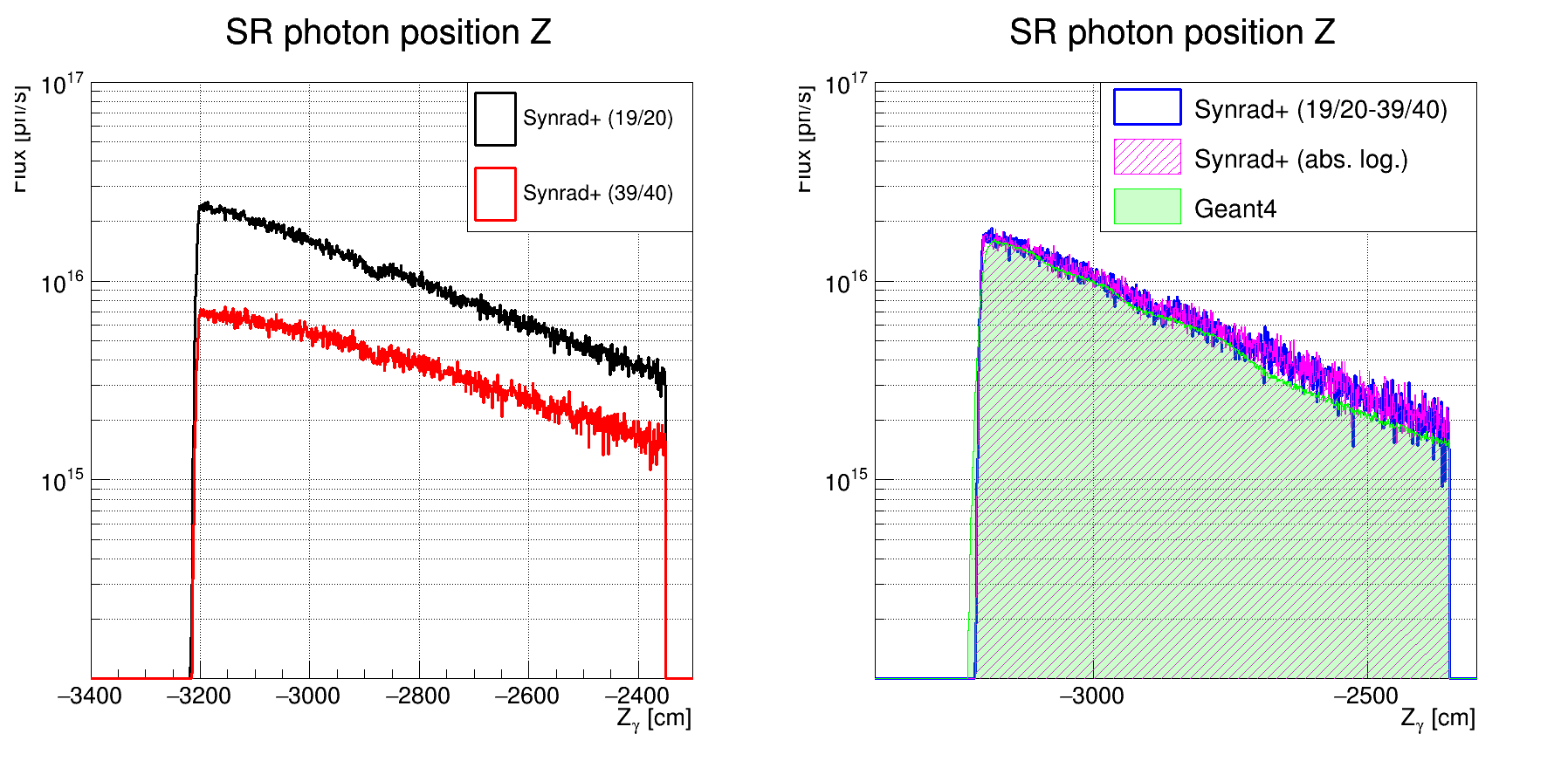
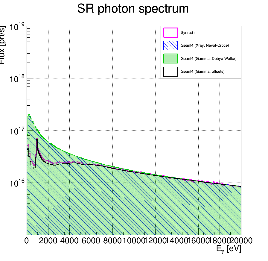
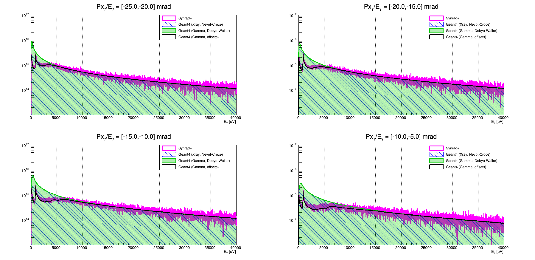
According to my results, it looks like the Synrad+ output flux of SR photons does not match my expectations based on the Geant4 code (page 2) and measurements (page 312, Table III - Copper).

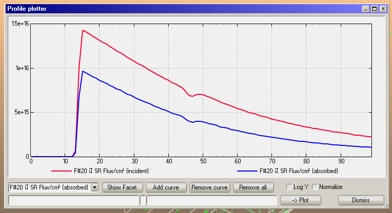
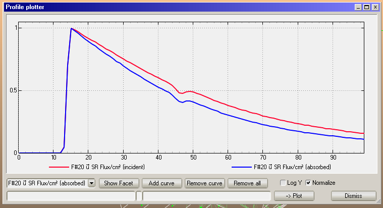
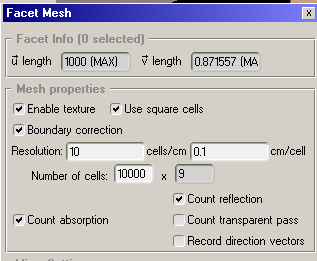
As one can see on page 4 (my doc), switching between the ideal absorber (sticking factor = 1) and a real absorber (02-Copper, roughness ratio = 0.005) for the vacuum pipe does not impact the absorbed SR photon flux vs horizontal incident angle.

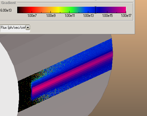
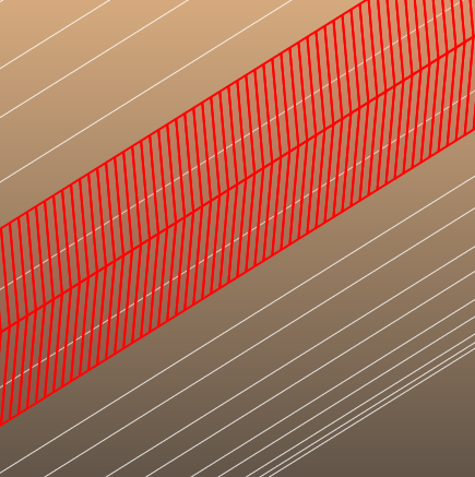
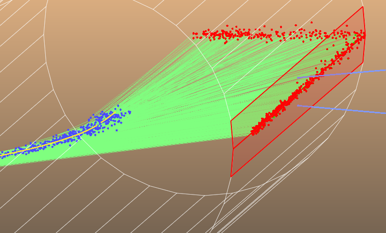
This analysis I did for only two facets with the highest SR flux from the 18 GeV electron beam passing through two dipole magnets with By = 0.2545244034 T.

Thus, could you please help me understand if it is a bug in Synrad+ (which I doubt) or my incorrect interpretation of Synrad+ results?

I appreciate any feedback you can provide.
Thanks and best regards,
Andrii

[rkerseva (Roberto Kersevan)]

Hello dear SYNRAD+ user, and tester.
Thanks for the nice message, document and analysis. Based on the information you’ve provided, I can’t tell you exactly what is wrong with SYNRAD+, if anything is wrong. I’d need the syn7z file as well, because “the devil is in the details”.
If you provide it, if it’s confidential you can send it to my e-mail address roberto.kersevan@cern.ch, I’ll be able to tell you whether the SYNRAD+ results you’re getting are correct or not… then why GEANT4 gives different results is another matter. I know from a recent workshop on FCC-ee MDI that H. Burkhardt is working hard on including photon reflection into GEANT4: is what you are showing here a similar independent development of yours, or is it part of a collaboration with him? Thanks.

[maarton (Marton Ady)]

Dear user,

Just a small thing to add to Roberto’s comment: if you share with us the file, please let us know…

• Which Synrad version you did your testing with
• Was “new reflection model” (in Global Settings) enabled? In newer versions this setting is saved with the file, in older versions it’s a program setting.

Synrad (and Molflow) had a design principle that you can run the simulations indefinitely, and it means that the memory and file size should not increase as the simulation goes. That’s why facets have counters (and profiles, textures) but you can’t individually extract the photon hits (except for the Particle Logger, which indeed means doing it one by one - it’s something that we might change in future versions, as others requested as well.

[andrii]

Dear @rkerseva and @maarton,

Thank you both so much for your prompt reply. I have prepared a ZIP file (synrad_vs_geant4.zip) with a simple geometry to reproduce my observation. You can download the file from here.

In the unzipped folder, you will find the following files:

• synrad_sim.syn – a Synrad+ script with simulation settings
• beam.bxy, D1.param, D2.param, and D3.param – region’s parameter files (three dipole magnets)
• facet_19_1M_particles.csv and facet_20_1M_particles.csv – stored particle fluxes on facets 19 and 20 (1e6 particles/facet)
• plot.C – a simple ROOT script to read the CSV files, convert them to histograms (storing into synrad_data.root), and plot distributions (saving as c0.png and c1.png)

The most crucial distribution is shown on c1.png (top, left plot – Flux vs Px/E). It illustrates a flat distribution (-0.025 < (Flux vs Px/E) < -0.005) for absorbed SR photons on the given facets, while according to my expectation, there should be some angular dependency. Please let me know if you have any problems accessing the files.

Answering your questions:

1. Unfortunately, I’m not familiar with H. Burkhardt’s work. I’m working on my independent project. But I think it would be great if, at some point, X_ray reflection would be available in the Geant4 physics process list.
2. I use Synrad+ version 1.4.32, released on Feb 20, 2023.
3. In Global Settings, “new reflection model” is not enabled, but I tried it and got the same results.

Thank you so much for considering this topic. I appreciate your help.
Best regards,
Andrii

[maarton (Marton Ady)]

Dear Andrii,

Thank you for the files and the benchmarks.

Before answering to the original question, one remark is that Synrad has built-in spectrum plotters, and they follow the general plot rule that the energy bins are variable, always equal to .1% of the energy mid-value. In your geometry, the plots therefore have a slightly different shape than in your files that you shared.

When using the spectrum plotter, you can distinguish incident and absorbed spectrum, see here on facet 20:

You can see a very clear difference between the incident (red) and the absorbed (blue) curve.

Unfortunately, I don’t know what the Rebin() command does in your script, and thus your bin size, so I can’t convert it to match the absolute values.

In any case, the particle logger records the incident hits, as I tried to suggest in the description:

In our terminology, “hitting” means all hits, regardless of the fate (absorption or reflection) of the particle. In other words, it is expected to not have any difference: you are simply doing statistics on the incident photons, which are normal to stay constant regardless of surface properties.

One remark about your regions is that it’s better to limit the generated energy to the spectrum (1…1e6 eV) for more resolution:

to

(or even to 20keV if that’s the spectrum you’d plot).

Can you maybe use the spectrum plotter, and let me know the bin size you used? Otherwise, if you need data for every hit, there are hacks to get only the absorbed data.

Cheers, Marton

[maarton (Marton Ady)]

PS You can also use profiles to show the incident/absrobed flux along the pipe length:

When normalizing to the peak, you can see the angular dependence of the absorption that you missed:

If you’d like to debug the remaining discrepancies, as pasted below, please let us know a bit more on how to interpret your plots (I think the X axis units should be m or cm, not eV).

[andrii]

Hi @maarton,

Thank you so much for your reply.

Let me answer your questions:

1. The Rebin() function is a standard ROOT CERN function of the TH1 class; see here.
2. In my simple script, I tried to build a distribution of absorbed photons on the given facets by filling a 1D histogram and using PhotonFlux as a weight.
3. eV in Y/X_gamma[eV] is a typo. It should be [cm].

Based on your explanation, PartileLogger does not give me the information I need since it stores the information about the incident photons, not absorbed. Therefore, could you please tell me about the hacks to store the information (i.e., energy, flux, XYZ position, XYZ direction) of absorbed photons for a facet?

I need this info because, in the next step, I will use the absorbed photon information and propagate it to Geant4 for the whole detector simulation (i.e., hit rate simulation). So, knowing only an energy spectrum of absorbed photons is not enough for my task.

I would really appreciate any help you can provide. Thank you in advance.
Best regards,
Andrii

[maarton (Marton Ady)]

Hello Andrii,

Some remarks:

1. While weighing by flux is correct, since you used “Fluxwise” mode, each line (virtual photon) represents the same weight (3.88E12 in your attached file).
2. You can use textures (color maps) for the spatial distribution
   
   2b) The texture can either record all flux (absorbed + reflected enabled) or only absorbed photons (absorbed checkbox only):
   
3. You can not, indeed, get the spectrum AND the flux for each texture cell.

Your options are:

1. Use the Mesh and Explode commands to partition the target facet to strips or squares, where each can have its own spectrum:

Then you can export the flux data from the facet list (lower right corner or facet details):

And the spectra from the .syn file (one column per facet, I can help with the exact interpretation):

Or you can create a transparent “capture facet” recording the reflected hits, as follows:

1. Select facets 19 and 20
2. Use the facet move to copy+shift them a tiny bit to the left (by 0.01cm for example)
3. Swap the normal of these facets to face the reflecting copper wall
4. Set their sticking to 1, to capture directly refelcted photons, and not the subsequent hits after bounces from the opposite wall, and enable particle logging.

This will work because these new facets (39 and 40) are 1-sided, meaning they let the photons through from their back, but capture the reflected ones:

This way you can log the reflected particles on these new facets and the incident ones on the original facets. It is up to see whether this helps to calculate the difference (absorbed), or not, because you’re not sampling exactly the same photons but two random statistics (even if the same size).

I attach a file as example:
synrad_sim_count_reflected.syn7z (71.7 KB)

Regarding the Rebin(100); command, do you confirm that your spectrums use 100 equal-sized bins of 200eV width each?

[andrii]

Dear @maarton,

Thank you! I will try to follow your suggested steps for at least the two facets, comparing them with my expectations.

Regarding Rebin(). In my script, I load a histogram TH1D* h1_ene_sr = (TH1D*)file_sr->Get("h1_ene_sr"); from the ROOT file, which was previously created as TH1D* h1_ene_sr = new TH1D("h1_ene_sr","SR photon spectrum;E_{#gamma} [eV];Flux [ph/s]",1e6,0,1e6); . It has 1e6 bins within 0 eV and 1e6 eV, which means 1 bin = 1 eV. And then I rebin it as h1_ene_sr->Rebin(100);, which means changing the number of bin from 1e6 to 1e6/100 = 1e4, so each bin is 100 eV now.

Cheers,
Andrii

[maarton (Marton Ady)]

Ok, thanks.
If the hacks above are too inconvenient, get in touch, and I can make you a custom version of Synrad, where the particle logger is only active for absorbed particles.
Let me know, Marton

[andrii]

Dear @maarton,

Again, thank you so much for your help. I decided to use option 2 with two additional facets (1-sided, sticking = 1, smaller radius). I collected all hits on my reflecting facets 19 and 20 (02-Copper), and all absorbed SR photons on the new facets 39 and 40. Then, I calculate the difference between the two distributions to get the absorbed spectrum on reflecting facets 19 and 20.

Fig. 1: energy spectrum of SR photons (in eV, 1 bin = 100 eV)

Fig. 2: SR position along the beamline (Z-axis in cm, 1 bin = 1 cm)

Left plot: black histogram – hits on facets 19 and 20, red histogram – absorbed photons on facets 39 and 40; right plot: blue histogram – the difference between black and red from the left plot, green histogram – Geant4 results. I used the old reflection model with a low flux mode (cutoff ratio = 1e-7).

There is now a much better agreement between Synrad+ and my Geant4 simulation. Of course, I cannot use Synrad+ option 2 for other distributions (e.g., angular), but I think it is already enough for my code benchmarking.

I think having a Particle Logger with an option of storing only absorbed photons would be helpful for other users, especially for those who want to study the spatial distribution of absorbed SR photons.

Thank you so much for your help. I believe the problem is SOLVED, and we can close this TOPIC.

By the way, I have noticed one issue related to the number of scans (Scn) and ParticleLogger when running the Synrad+ simulation. If I set (for example) 1000 particles to log and then press the button Begin, the logger starts collecting hits in the given facet until the specified number of particles is reached, let’s say at Scn=20, but the simulation is still running. Then, after 2-3 seconds, I press the button Pause at Scn=30, the simulation stops, and then I export the stored/logged particles to a CSV file. The problem is that the exported flux of particles (as far as I understand) is normalized by the number of scans (Scn). And since I stopped the simulation at Scn=30, not Scn=20, the exported flux is normalized by the wrong number. So, to get the correct normalization, I had to simulate during a fixed time (for example, 10 or 20 sec) with the max recorded/logged particles set to some huge number (for example, 1e6) to be sure this counter is not exceeded.

Best regards,
Andrii

[maarton (Marton Ady)]

Dear Andrii,

I have released Synrad 1.4.33 which has the option to log only absorbed particles.

If you have the time, maybe you can benchmark the previous test case, and check if the results are the same as with the hack (incident minus reflected).

As for the number of scans problem, you’re right, but it is very hard to fix with the current Synrad architecture.
The problem is that the particle log is written by the “worker” subprocesses, which are not aware of the global simulation state (summing the partial hits recorded by the workers, and normalization is done by the GUI). In other words, the represented flux and power is a derived quantity, which requires the state of the other workers.

I did an approximate fix as follows: when the particle logger reaches the log limit, it remembers the number of scans in that update, and uses that remembered number to normalize. It is not perfect:

• State synchronization happens once per second. If the log is exceeded by a large amount during this second (for example, update from 900.000 to 1.100.000 recorded particles), then the remembered “number of scans” will correspond to 1.100.000 hits, not 1.000.000.
• You can disable the scene auto-update in Synrad, in which case the limit will be simply missed.

That said, for regular cases, when the particle log increases slowly, it should be a much better approximation than the previous version (which always normalizes with the current number of scans).

I hope this best effort fix, that’s now in the new version, is acceptable, and thank you again for the bug report.
Cheers, Marton

[andrii]

Dear @maarton ,

Thank you so much for preparing a new release with improved features.
After downloading MacOS binaries for the new release v1.4.33, I ran the simulation with my geometry and observed one strange behavior for the Particle Logger:

1. When I select only “Enable login,” everything works as before,
2. When I select “Enable login” and “Log only absorbing particles,” the Logger does not store any information; see below.

Is it an issue on the Synrad side, or did I do something wrong?
Thanks,
Andrii

[maarton (Marton Ady)]

That’s strange, I tested with your geometry, but i obviously did something wrong. I am currently out of office but will have a look asap on Wednesday and get back. Cheers, Marton

[maarton (Marton Ady)]

Hello again Andrii,

I played around and I believe you have low flux mode enabled.

• In regular mode, Synrad decides if a particle is reflected or absorbed.
• In low-flux mode (see details in 5.4 of https://molflow.web.cern.ch/sites/default/files/synrad_docu.pdf), all particles are reflected, however the reflected part will represent a lower flux.

(You can toggle low-flux mode in Global Settings)

Since in this case no particle gets absorbed, the particle logger doesn’t log anything in absorption-only mode.

In a future version I will change this to still log absorptions, just with the “oriRatio” column reduced from 1 to a lower number represeting the absorbed part.

[maarton (Marton Ady)]

PS I’ve compiled a temp version with the low-flux logging enabled for absorbing particles, you can download it from the “build-artifacts” column for your OS:

Pipeline · molflow_synrad / synrad · GitLab

[andrii]

Dear @maarton,

Thank you so much for preparing the temp version with the low-flux logging enabled for absorbed particles. Indeed, it helps, and now I see perfect agreement between the “hack” (blue histogram) and “new release + low-flux log.” (hatched magenta histogram) results; see below.

I’m still trying to understand the discrepancy for the low-energy part of the spectrum between Synrad+ and my Geant4 code. I have to do a more detailed study.

Cheers,
Andrii

[andrii]

Dear @maarton,

Coming back to the Synrad+ and Geant4 comparison for X-ray reflection.

Since X-ray reflection as a standard gamma process was missing in Geant4, the Geant4 developers have recently (Dec. 2023) implemented this process; see #50 FCC-ee MDI meeting

• They use the same material reflection database (like Synrad+) prepared by B.L. Henke et al.
• Unfortunately, they consider only specular (mirror-like) reflection with an attenuation factor to include surface roughness.

So, I adopted the released Xray process from Geant4 and compared the following codes:

1. Synrad+ (using the recently prepared version with a bugfix and absorbed photon info; see this topic) – diffuse reflection
2. Custom-built Geant4 code

• With the Debye-Waller attenuation factor – specular reflection
• Without the att. factor but with the reflection angle offset (from here) – diffuse reflection

3. Geant4 release with the Névot-Croce attenuation factor – specular reflection

I used the same reference facets, #19 and #20.

For roughness = 0 nm, I got a good agreement between all models; see the attached page-1.

Then, I put roughness = 50 nm and roughness ratio = 0.005 (old reflection model). I got a perfect agreement for specular reflection between custom-built (Gamma, Debye-Waller) and release (Xray, Nevot-Croce) Geant4 models, but there is a noticeable disagreement for diffuse reflection between custom-built Geant4 (Gamma, offset) and Synrad+; see the attached page-2. By putting roughness ratio = 0.005, one can see that the reflection probability for low energy SR photons (E < 6 keV) changed in Synrad+. In contrast, only the reflection angles should be changed according to Documentation.

Furthermore, in the Synrad+ software help window, there is the following info:

. As far as I understand it, in the old reflection model, the material reflection probability depends on the surface roughness. Could you please share the info on how exactly it depends? Do you apply additional attenuation factors?

I appreciate any help you can provide.
Best regards and a Happy New Year,
Andrii

page-1

page-2

[maarton (Marton Ady)]

Hello Andrii and many thanks for benchmarking.
I have followed H. Burkhardt’s presentation, and found this page that compares the Debye-Waller and Nevot-Croce: Optica Publishing Group

Citing from that page:

The Névot–Croce and Debye–Waller factors correct the Fresnel coefficients of an interface according to its roughness. The former is used for approximating the effect of roughness that has high transverse spatial frequency, where diffuse scattering is negligible. The latter is used for roughness with low transverse spatial frequency, where diffuse scattering is located very close to the specular reflection.

For your info, I chose to use the Debye-Waller as I’m basing my model on that of Synrad3D (Cornell, Dugan and Sagan, described here: https://cds.cern.ch/record/1668186/files/Dugan-II-edited.pdf)

I believe that in accelerators, it is not correct to assume that diffuse scattering is negligible: photons travel downstream large distances and reach the surface in very low grazing angles (almost parallel). Therefore I’d defend Dugan and Sagan’s choice to apply the Debye-Waller and not the Nevot-Croce factor.

Here is an excerpt of the old and new models:

Old reflection model:

• First perturbate surface normal according to “roughness ratio”
  • If incident shadowing (ray would come from behind), repeat by generating a new random tilt angle
• Treat everything else as if the surface was locally flat
  • Calculate incident theta with perturbated surface
  • Look up reflection probability (function of theta and energy)
  • Specularly reflect on perturbated surface
  • If outgoing shadowing (going against original surface), generate new perturbated surface and do everything again

New reflection model:

• Calculate incident theta with original surface
• Get reflection probability (support for transparent and backscattering)
• If reflected:
  • Calculate Debye-Waller factor (depends on roughness, energy and incident angle)
  • If specular reflection based on Debye-Waller factor, reflect in perfectly specular manner
  • Otherwise perturbate reflected angle based on roughness and autocorrelation length

I have benchmarked the new model both for the Debye-Waller reflection probability (aligning tiny targets that measure the perfectly reflected part):

And also the angular pattern of the diffuse reflections:

So I consider the “new model” phyisically sound and documented.

It has one problem, though: as Synrad+ uses polygonized geometries, the perfect reflection probabilities result in “artifacts”: since curved walls are represented as polygons, the reflected pattern is not smooth.

The old model, ported from an earlier code, without any physical model to back it up, smoothes out these. That said, although benchmarking was done to match the new and the old models, they work differently and cannot be matched. It is expected that the old model results in different reflection patterns, and also that due to perturbating the local surface, they change the reflection probability. Long story short, the new model should be used - I’m happy that you’ve found good agreement woth Geant4.

PS Could you please drop a few lines (here or to marton.ady@cern.ch) to introduce yourself? I’m in occasional contact with H. Burkhardt and your benchmarking is quite useful - it would be nice to refer to it, knowing who you are and which institution or experiment you work for. Many thanks!

[andrii]

Dear @maarton ,

Thank you for these explanations. And special thanks for listing all the steps behind the old and new reflection models in Synrad+.

Initially, in my custom-built Geant4 code, I did not perturb the surface normal, only the reflection angles. However, after your recent details, I modified the code to perturb the normal (this, of course, affects the reflection probability) and treated everything as a specular reflection. Indeed, that improved my results, making them very close to Synrad+; see the attached pictures.

Fig.1: Energy spectrum of absorbed SR photons by facets #19 and #20. There is a good agreement between Geant4 codes for specular reflection (blue hatched and green) and Synrad+ vs Geant4 code for diffuse reflection (magenta and black). Surface roughness = 50 nm and ratio = 0.005.

Fig.2: Energy spectrum of absorbed SR photons by facets #19 and #20 for different incident angles in the horizontal plane. There is good agreement for all angles. Surface roughness = 50 nm and ratio = 0.005.

Fig.3: Angular and spatial distributions of absorbed SR photons by facets #19 and #20. Surface roughness = 50 nm and ratio = 0.005.

• Magenta histogram – Synrad+ simulation results → diffuse reflection (old model)
• Blue hatched histogram – custom-built Geant4 code adopted from geant4-release-11.2.0 with a Névot-Croce attenuation factor → specular reflection
• Green histogram – custom-built Geant4 code with a Debye-Waller attenuation factor → specular reflection
• Black histogram – custom-built Geant4 code with a randomly tilted reflection surface normal → diffuse reflection

So now, I have a single flag in my code as an input parameter to choose which reflection model to use for the simulation. Also, I agree that the diffuse reflection is better for the accelerator vacuum beam pipe since accurate SR photon tracking along the beamline is essential, especially for the IP section.

To implement the new Synrad+ model into my custom-built Geant4 code, I have to develop a code for the last step in your new-model list: “Otherwise perturbate reflected angle based on roughness and autocorrelation length”. This will require the calculation of the diffusely reflected power fraction as discussed here. As far as I understand, you use some approximation with fit parameters. Perhaps I should follow the same strategy. Please let me know if you have any advice. Do you have any updated fit parameters, or are the published numbers in your thesis still valid?

Also, could you please tell me how you ended up with the two equations for the perturbed surface normal?

thetaOffset=atan(sigmaRatio*tan(PI*(rnd()-0.5)));
phiOffset=atan(sigmaRatio*tan(PI*(rnd()-0.5)));

For the moment, I plan to use my custom-built Geant4 code with a diffuse reflection based on the perturbed surface normal, so-called “Geant4 (Gamma, offsets)” – black histogram. Maybe later, I will improve it following the new Synrad+ model.

I will contact you by email to introduce myself.

Thanks and best regards,
Andrii