Validity of Molflow simulations

Hello all,

Although Molflow+ is an attractive software for vacuum system simulations, I am concerned about the validity of the outputs. I tried to evaluate the conductance between the main chamber and the pumping station in my system using Molflow+. Moreover, I simulated the pressure distribution in the chamber to evaluate the pressure difference between different parts of the system. How can I ensure the validity of these results?

Thank you

  • You would first try to reproduce known conductance results and see if Molflow’s result is the same.
  • Then you would do the same with simulating known pressure distributions.
  • Then you would read the algorithm and compare it with textbooks: The algorithm behind MolFlow+ - MolFlow+ / SynRad+ documentation
  • Finally, Molflow is open source, you can check how it works on every level.

Dear Marton,

Thank you for your response.

Do you have any information about the error in the simulation outputs? For example, suppose I have simulated a vacuum chamber and used Molflow to calculate the particle density in a specific region of the chamber. Do you know the percentage error of the results obtained, assuming that I have accurately entered the system parameters such as geometry, pumping speed, and outgassing?

For the detailed reply, see section 1.2.1.9 on page 23 of my thesis.

Since I wrote the thesis there’s a new tool called convergence plotter to see the percentage value in an actual simulation, in your example you’d create a formula for the density first, for example DEN123 is the density on facet 123.

The transmission probability calculation has an associate standard deviation (binomial distribution) given by an analytical formula: if p is the transmission probability, then the “true value” will be contained in the band given by

P_tr = p +/- (sqrt(1-p)*p/N_tr)

where N_tr is the number of TRANSMITTED molecules.

So, if you have P_tr=50% you need to have N_tr=2500 in order to have sigma=1%.

Sigma goes with the square of N_tr, so to reduce sigma by a factor of 10 you need to run 100x longer the simulation. This is why TPMC is sometimes avoided and alternate methods are used. If your p is very small, i.e. N_tr/Ntot is small, you’d need to run the simulation for a very long time, or use a powerful computer. In literature you can find people who do that routinely, like those at KIT in Karlsruhe, on their ProVac3D code (similar to Molflow+) which has been adapted to run on GPU-based parallel supercomputers ("Marconi, in Italy).

Therefore, for a given geometry, and therefore p value, you can calculate how many N_tr molecules you’ll need to generate before you reach a statistical error of x%, by reversing the formula above.

More details for instance in this excellent paper:

https://pubs.aip.org/avs/jva/article/14/1/245/318120/Application-of-the-Monte-Carlo-method-to-pressure

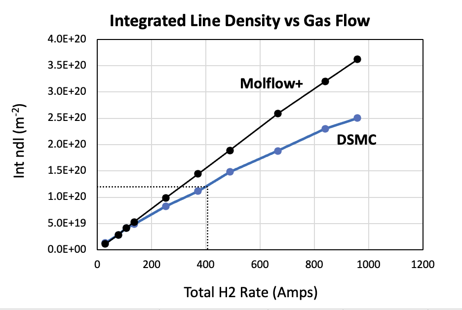
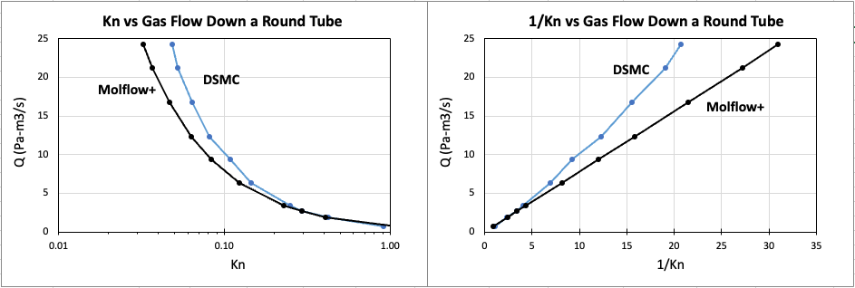
I have personally validated tens of calculations/measurements found in literature, when sufficient details had been made available that allowed me to make a Molflow+ model of the system discussed in the articles, and I have always found a very good, if not perfect, agreement with those data. The only deviations start to be visible when the mean-free path comes close to the Knudsen regime, also called transitional regime, the one that connect the free-molecular flow region to the viscous flow one. I have shown some examples throughout the years on various occasions, mainly workshop and conference presentations… unfortunately I do not have now the time to link them here, sorry.

Summary: based on decades of use of the code, you can safely assume that its output is correct. This means, though, that the geometrical model you built and the physical assumptions/properties you assigned to it are a faithful representation of the real physical model.

I’ve used DSMC to accurately simulate transitional flow down a simple round pipe and I compared it to Molflow. Molflow gave about a 25% higher density in the pipe, so it’s not a bad first approximation if you just need a ball park number. FYI “ball park” is American baseball slang for being approximately close.

Hi Alan, and thanks for the feedback on DSMC vs TPMC.
May I ask you for which Knudsen number (or range of Kn) did you find this 25% agreement between the two?
Thanks.

Roberto,

Here is a comparison plot of flow rate vs integrated line density (along the length of the tube). It was a 39cm diameter tube x 1.75m long. If you divide this by the length you will get the average density in the tube and from that the average Knudsen number. For the integrated line density I needed, I think the pressure was in the 2-3mTorr range, but also keep in mind my gas temperature was 500K, so equivalent room temperature pressure would be lower. Also, I find doing flow in Amps convenient, so just divide by the electron charge (1.6E-19) to get the rate in #/s. It’s easy to mix up what temperature you are refering to when working in PV units like mBar-L/s. Usually, room temperature is assumed but my gas is at 500K so you might input the wrong value into Molfow.

Best,
Alan

OK, a bit too many conversions to do from very unusual units, but thanks anyway Alan!. :slight_smile:

39 cm ID is huge, so at a relatively high density the MFP is certainly smaller than that, and therefore the Kn is large.

I remember replicating studies with Kn of a few units, i.e. transition regime, and one could barely tell the difference with TPMC.
I’m trying to remember which paper it was, though, it is somewhere on the backup I made before leaving CERN.

What units do you want. It will only take me a couple minutes to create a plot for you.

I think you mean Kn is really SMALL. Kn=Lamda/Dia. Maybe these plots are more what you want…

Yes, my bad… Kn is SMALL for small Mean Free Path, obviously.
Thanks for the two plots.