Hello there. I’m using molflow 2.8.10 and am having some weird behavior modeling temperature for my vacuum system. Im injecting gas at 650 K into a region and is being pumped out at various places. The gas and the walls of the system are in Thermo equilibrium, and there is no external heat being added to the system. Since I couldn’t find a way to plot Temperature in the transient simulations, I take the pressure graph and the density graph and use P=nkT to solve for Temperature.
The setup of the problem is as follows:
*from t=0 - t=0.001 gas is slowly injected from the walls until the system reaches a pressure of 1E-5 mbar. Once it reaches this pressure the slow gas injection stops.
*from t=0.001 - t=0.003 gas is puffed into the system through a gas valve.
*from t=0.003 - t=0.1 all outgassing sources stop and pumping is the only thing left.
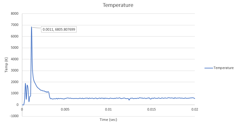
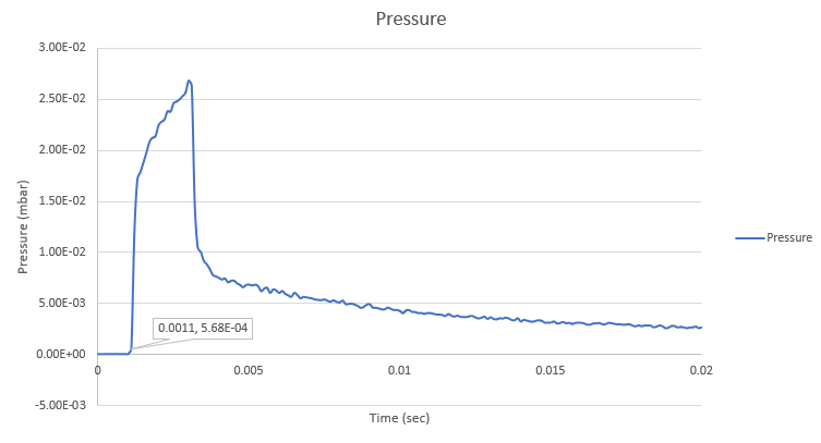
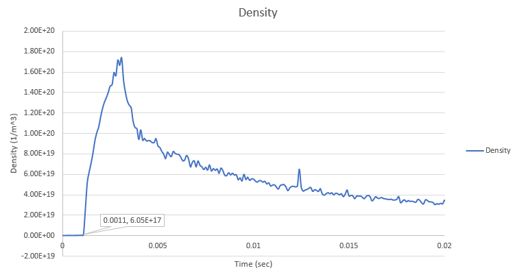
In the graphs bellow, what I’m experience begins at the moment gas puff is injected (t = 0.001 seconds), and at 0.0011 seconds there is a huge temperature spike to around 7000 K. The gas is only at 650 K and I should expect the gas to be at its maximum temperature the moment it is injected and then reduce from there. I’ve tried bunches of different moment settings to resolve more and resolve less, but In my problem I just keep getting the same result but slightly different values depending on the # of moments. Any idea what might be going on here? I think it might be a issue with a lack of numerical resolution in the monte carlo, but im not sure.
Hello Skyler, congrats on setting up a time-dependent outgassing and simulation which isn’t easy.
The p=nkT equation is valid for ideal gases, notably in cases where the gas is more or less in equilibrium and is isotropic.
This is true during a slow injection (0 to 1 ms) but not during a sudden puff, where molecules move away from the inlet valve until they thermalize through wall bounces and fill the volume evenly.
The other issue is that density is scalar, but pressure isn’t: it depends on the direction (it is derived from molecular forces, which are due to impulse change on a surface, and impulse contains velocity, which has a direction). You can test this by rotating your sampling surface: you will see that Molflow always measures the same density regardless of facet orientation but the pressure will be larger when sampled perpendicular to the injection than parallel to it. Again, most textbooks describe the equilibrium (isotropic) case where the direction doesn’t matter.
There is no way to visualize temperature better than what you did, since temperature is, after all, a statistical parameter derived from the velocity distribution of the particles. You can, however, sample time-dependent velocity distributions (with the “speed” profiles) and analyze that yourself.
If you’d like, I can have a look at your ile to confirm if this is the case (anisotropy).
Otherwise, maybe we can figure out together what and how to measure, depending on what the goal is.
Hi Marton, thank you for the explanation. The goal of what i’m trying to measure is conduction over time. Since the conduction of an orifice is related to the sqrt(T) I want to graph the change in conduction of two different orifices’ in my system. I’m thinking that maybe the molecular velocity works? I could take V_avg_mol = sqrt(8RT/piM) and solve for T. In facet details it gives the molecular velocity, but it seems like its giving the avg molecular velocity over the whole facet at each moment. Though I’m not sure how to export that data from the program
I could also export the speed plots from the profile plotter, however I don’t know how to export every plot for every time t.
Make sure you have the Surface->Volume conversion enabled (you’d like to sample to speed distribution in the gas, not on the surface, the two are different).
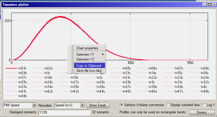
You can define which moments to export in the displayed moments textfield:
1,1,50 displays 1,2,3…50
1,5,101 displays 1,6,11,16…101
And so on.
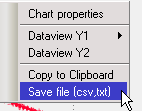
To export (instead of display) right-click and copy to clipboard or save as file:
From the distribution you can get the average velocity, then the equivalent temperature.
Two remarks:
The average velocity in the facet details window is not exactly measured (as facets don’t have the specific counter required for this), but is just an estimation assuming ideal gas. That’s why the profile plotter is exact, and to be used.
If you only look for the conductance over time, the temperature calculation might not be necessary, since in isotropic conditionsC=0.25*<v>*A where <v> is avg. mol. velocity and A is the orifice surface. This is not true in anisotropic conditions (the factor of 0.25 is the fraction of molecules moving towards the orifice when integrating over all possible directions and velocities, and is derived assuming isotropy). In anisotropic case, you would need the distribution of the orthogonal velocities (moving towards the orifice), which Molflow can measure (there is a profile option for that), but I admit I don’t know how to derive the conductance from that.
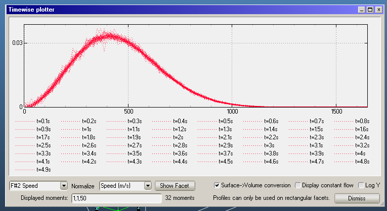
Thank you for the help Marton. I’ve got a plan on how to tackles this now. I’ve been wondering however about the speed plot inside of the timewise plotter. Im assuming in the graph the X axis is speed (m/s) and each line represents a time t, but what is the Y axis? It doesn’t look like pressure, but maybe its a normalized location on the facet? I’m not really sure and was just wondering what exactly that axis was.
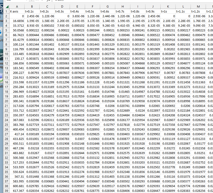
On a helper sheet, calculate the bin centerpoints (center speed) with an extra column
Calculate the weights as bin_center_speed * bin_weight
Calculate the weighted sum of of each column (SUM of weights).
So you can see that the average speed at every moment.
I attach an example Excel file where you just have to paste the raw data from Molflow to the first sheet. timedep_example.zip (170.4 KB) mean speed calc.xlsx (142.9 KB)