Dear Marton and Roberto
I have one question while doing time-dependent simulation. For example, I set the time moment as [1e-4, 1e-4, 0.1]s. To inject a given number of particles to a volume, I stop outgassing at a certain time (0.0001001 s). Then I can obtain the target outputs at different moments, like the MC hits of each facet. I know that Molflow use a smaller number of virtual (test) particles to represent the real number. My question is: whether the number of virtual (test) particles will change when the simulation is running? At a certain time moment (0.1 s), when I click the update button, the MC hits keep growing. if the virtual (test) particles does not change, the MC hits should keep constant at a certain time moment.
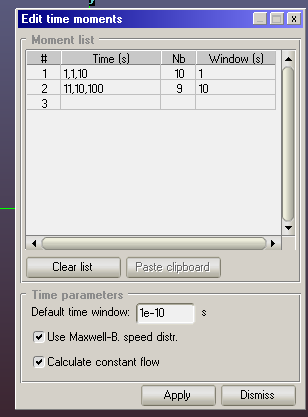
In addition, there are two time window in the time edit moment. which one is the parameter used in the calculation in Molflow?
Thanks for any feedback.
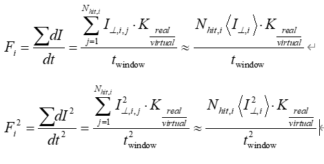
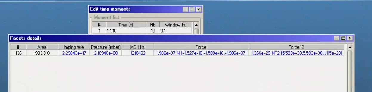
To inject a given number of particles to a volume, I stop outgassing at a certain time. So I obtain the corresponding result, as shown in attached file. I am confused about the ForceSqr. Firstly, I make a simple check to the Force result. According to the document, the force should be calculated by eq. (1). In this moment, the hits are 69442. Since the collision type is diffuse, so the average momentum is about m_0sqrt(2pik_bT/m_0). K_{real/test} can be calculated by the imping rate. The I obtain 0.002101 N, closed to the simulated result. For the calculation of ForceSqr, I think the equation should be eq. (2). Similar to the above calculation, the average momentumSqr is about m_0^2*{(4+pi)k_bT/m_0}. Inserting these parameters into eq. (2), the result is 6.5988*10^{-20} N^2. So I am not sure about the calculation in Molflow.
Thanks for any feedback.
- Yes, the number of test particles grows continously as the computer is calculating.
- The time window applied is the one at the end of each line. The “default” textbox is just a helper tool to pre-fill that value. In the example below the first 10 moments have window=1s the second 10 window=10s
I think the attached file is missing.
Your pre-conditioning method (injection q until time t1) is correct, for example an outgassing speed of q=10mbar.l/s in a 10l volume during 0.005s would result in a pressure of 0.005mbar (after the system has time to equalize).
The “ForceSqr” variable was added at the request of the LISA experiment, and they asked it to be defined as the sums of m*v^2 components. When calculating the quantity, the time window does not raise to the square in the denominator. If I understand correctly, your definition for <I^2> would be SUM((m*v)^2)/N, differing by a factor of m.
I can’t verify if this is the case, as I don’t know which gas mass and time window you’ve used.
It would make sense to change <I^2> to SUM(<m^2*v^2>)/N, and I can do that in an updated version, but is there a physics reason to divide by dt^2 instead of dt?
(There is no “momentumSqr” variable)
Thank you, Marton
Sorry for the late answer, I am out of school recently. I have attached a PDF file. If you can not load it, please contact me.
Thank you.
file.zip (117.1 KB)
Dear Guest (sorry, I don’t know your name),
Before replying to other parts of the PDF, could you provide a reference or some further info on the sentence:
“The velocities in the normal direction obey the Rayleigh distribution”.
This is the first time I hear about this.
As far as I know…
In the volume
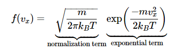
Each direction component in equilibrium obeys a Gaussian distribution:
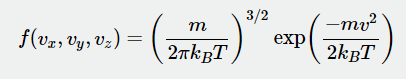
And the velocity (vector length) is the square-root sum of the three components, i.e. the Maxwell-Boltzmann distribution:
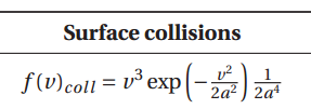
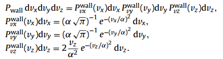
On a surface
Both distributions are shifted to higher velocities (need to be multiplied by v), as faster molecules hit a surface more often.
Do we agree on this?
Thank you, Marton
Dear Marton
Yes, each direction component in equilibrium obeys a Gaussian distribution before it collided with a surface. After collision, the reflect velocity in the normal direction is restricted. Many papers refer it as Maxwell-Stream distribution.
you can find it in Appendix of Ref 1[Suijlen M A G, Koning J J, van Gils M A J, et al. Squeeze film damping in the free molecular flow regime with full thermal accommodation[J]. Sensors and Actuators A: Physical, 2009, 156(1): 171-179.]
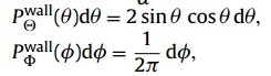
In fact, the method in your paper and the method in Ref 1 are consistent. For example, you generate the φ azimuth and θ angles as follows:
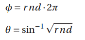
which implies that
then you generate the velocity
changing to the cartesian coordinates
therefore, the results are consistent.
can you see the figures that I inserted?
Thank you, Ke Jun.
Thank you Ke for looking into this and the detailed explanations.
I’m out of office until mid-next week, I’ll have a look on my return and get back to you,
Thank you for your patience, Marton
Hello again Ke, I had a look.
- I have fixed the calculation to divide by dt^2, as you correctly pointed out that it’s the correct way to get [N^2] unit in the result
- I previously wrote that I calculate force_sqr components as
m*v^2, but looking at the code I raised the mass to the square as well - in your calculation you do the same, this was just a minor thing.
This changes the result by the time window size (a factor of 1E-4 in your example).
For the discrepancy between your expected 6.63E-22N^2 and the simulated 4.63E-22N^2, I found that in your PDF, you calculate the average impulse like this:
However, I am squaring the forces component-wise in Molflow:

In other words, if
impulse = (m*v_x, m*v_y, m*v_z)
then
impulse^2 = (m^2*v_x^2, m^2*v_y^2, m^2*v_z^2)
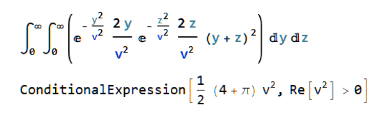
In the PDF that you attached, (y+z)^2 should be changed to (y^2 + z^2)
Once again, the component-wise squaring was chosen somewhat arbitrarily, is there a convention or a physical reason to do it differently? (The exact way to square a vector is not trivial)
Dear Marton, thank you for your reply. When I change the (y+z)^2 to y^2+z^2, the result is right.
For example, the velocities in x direction before collision and after collision are v_1 and v_2, respectively. You recorded the impulse^2 as m^2*(v_1^2+v_2^2) in your code?
Yes, as you write.
Impulse: m(v_1 - v_2)
Impulse^2: m^2*(v_1^2+v_2^2)
Where v^2 is componentwise squaring.
Dear Marton, thank you for your quick reply. Then we can discuss the way of the component-wise squaring. In fact, the “ForceSqr” variable is used to calculate the power spectrum density or the damping coefficient. The related article is [ Cavalleri, A., et al. Gas damping force noise on a macroscopic test body in an infinite gas reservoir. Physics Letters A 374.34 (2010): 3365-3369.].
Let me explain the details of our target result. For example, there are N_all molecules in this simulation. The simulation time is 0-T_end, maybe t_window will not needed in our scheme. For 1st molecule, it will collision with the target surface i many times, such as N_coll during the [0, T_end] interval. I will record the sum of the N_coll impulses. Then repeated for N_all molecules. therefore, i can obtain a 1*N_all vector FF. Finally, the “ForceSqr” variable is calculated by FF(1)^2+FF(2)^2…+FF(N_all )^2. I know that this procedure is not compatible with your current code. But I think it is easy for to realize this problem. This is also the procedure of LISA.
Thank you.
Ke Jun
Hello again Ke,
I’ve read the paper, thank you. However I don’t understand the mechanism that you describe (or I don’t see how or where it’s described in the paper).
Would changing impulse^2 to ( m*(v2-v1) )^2 from the current solve your request, or the process you describe is different?
Thank you, Marton
Hello Ke Jun,
I’m currently researching mass block force noise in gravitational wave detection. I’m a bit confused about using “forceSqr” in Molflow reference documents and your mention of it for calculating Brownian noise. My understanding was to collect the time-domain signal of the total force along the sensitive axis of the mass block and then obtain its power spectral density to determine the force noise. However, it seems like “forceSqr” is not utilized in this process. After reading the Molflow documentation and your posts, I suspect my understanding is incorrect. So, I would like to ask you how to use “forceSqr” to calculate force noise. I’d appreciate it if you could provide some details or direct references. Thank you very much!
ke jun,您好,
最近我在做引力波探测中质量块力噪声方面的研究,我对molflow参考文档和您提到的用”forceSqr"来求布朗噪声不是很理解。在我的理解中,采集到质量块敏感轴方向的合力的时域信号后,在求出这个合力的功率频谱密度,就是质量块受到的力噪声,但是这似乎没有用到“ForceSqr"。通过阅读molflow帮助文档和您的帖子我想我的理解是错误的。所以,我想向你请教如何用“ForceSqr"求得力噪声,烦请您尽量告知我一些细节,或者给予一些直接的参考文献。不胜感激!
Hello Marton,
I’m currently researching mass block force noise in gravitational wave detection. I’m a bit confused about using “forceSqr” in Molflow reference documents and Ke-Jun mention of it for calculating Brownian noise. My understanding was to collect the time-domain signal of the total force along the sensitive axis of the mass block and then obtain its power spectral density to determine the force noise. However, it seems like “forceSqr” is not utilized in this process. After reading the Molflow documentation and Ke-Jun’s posts, I suspect my understanding is incorrect. So, I would like to ask you how to use “forceSqr” to calculate force noise. I’d appreciate it if you could provide some details or direct references.
Thank you very much!
ForceSqr is the square sum of the force components: m^2*(v_in^2 + v_ou^2)
Ke suggested to change it to m*(v_out-v_in)^2, but didn’t follow up, I guess he didn’t need to use the feature.
You would need to look at the temporal evolution of ForceSqr to calculate the noise. The feature was added at the request of a researcher from the LISA experiment, you’d need to do the research for the details as I didn’t use the ForceSqr, just added it to MolFlow on request.
Hello Marton,
Recently I read some papers about how to use ForceSqr to calculate gas noise,including paper Ke mentioned.I think Ke’s suggestion based on the equation in this paper.(“Gas damping force noise on a macroscopic test body in an infinite gas reservoir”)

However,I met a problem when use the forcesqr( get by molflow ) to re-calculate the data in another paper.(Brownian force noise from molecular collisions and the sensitivity of advanced gravitational wave observatories).
As you can see,ForceSqr in z axis is 1.115e-29 N^2,time window is 0.1s, pressure is 2e-6pa,same pressure with paper.
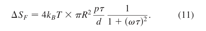
Use the equation in the paper,I can get S0(also SF0)
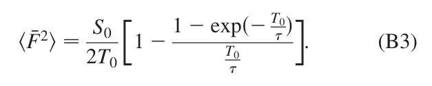
T0 is time window ,“tau” is escape time. In my simulation d is 5mm,“tau” is 5.64e-4s.
Then I want to calculate the Sf(w) to compare with paper.However,when calculate delt(SF0),I got a nagetive value,which is theoraticly impossible.
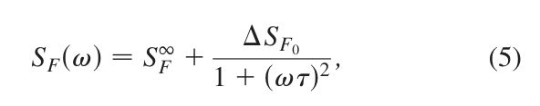

Also I use this equation to calculate Sf(w) in low frequency directly,the data is not compatible.Paper is 1e-14,mine 1e-15.
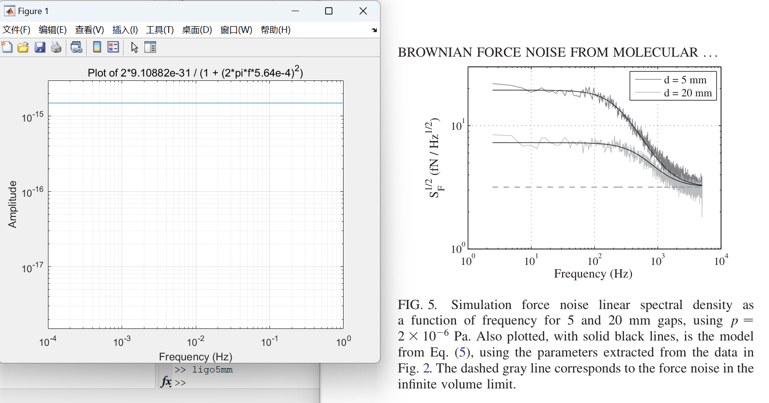
And paper’s data is wonderful compatible with another model
I think there is some differernt with molflow and paper to calculate ForceSqr. Maybe Ke’s suggestion is right?
If you have any interest to re-calculate the data,you can just use equation 1-7,11 and appendix B in this paper(Brownian force noise from molecular collisions and the sensitivity of advanced gravitational wave observatories).
All the papers and my molflow model are attached below.
Thanks in advance!
Brownian force noise from molecular collisions and the sensitivity of advanced gravitational wave observatories.pdf (604.2 KB)
Gas damping force noise on a macroscopic test body in an infinite gas reservoir.pdf (193.4 KB)
ligo-5mm.zip (1.6 MB)
Dear Wang,
In conclusion, what change do you suggest to do to the ForceSqr calculation method?
Thank you, Marton
Dear Marton,
After reading paper carefully,I think the method in molflow calculating forcesqr is right.The reason for the simulation results different with paper may be the follows:
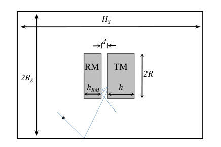
R=17cm Rs=10R d=5mm&20mm h=20cm hrm=13cmm Hs=11h+hrm+d
The author sets a simulation time T0 (e.g., 0.1s), assigns a random initial position to a particle within the entire chamber, and allows the particle to move within the chamber for the duration T0. Only the momentum exchange between the particle and the two bottom faces of the TM, as well as the square of the momentum exchange, are recorded (since the particle collides with more than just these two faces during its motion). By calculating the average for N particles, the total momentum exchanged with the TM by each particle is obtained.
I’m wondering if Molflow is capable of performing this function.
Thanks in advance!
Yes. The only part that can’t work out of the box is the random initial position of the test particle.
For that, the simulation has to start earlier, releasing a Dirac delta (a built-in time parameter) burst of particles, then run until those particles uniformly fill the volume.
Molflow records force, not momentum, but the quantities are convertible if the time window (dt) is known: dI/dt = F